Software¶
Most software on the Hoffman2 Cluster is available via environmental modules. A list of applications available via modules can be generated entering at the terminal prompt via the command:
$ all_apps_via_modules
or the module for a particular application can be searched via:
$ modules_lookup -m <app-name>
Some applications are available via python or mamba and will not be visible until a python or mamba modules are loaded. To request or suggest software installation or updates, please submit via our helpdesk. Only software/applications that is required by multiple groups may be centrally installed or you and your group will receive given guidance on how to perform software installation in your $HOME or, if applicable, in your group project directory.
Available software on the Hoffman2 Cluster organized by category is discussed below, for faster navigation use the menu (which, depending on your device, might be located in the sidebar or accessible via the collapsed menu icon: ≡):
Productivity |
Development |
Discipline |
|---|---|---|
Hoffman2 Cluster tools¶
A collection of commands designed to show the status of specific user attributes on the cluster. The commands are designed to be issued from a terminal connected to the Hoffman2 Cluster.
check_usage¶
check_usage is text-based command that allows users to monitor their jobs instantaneous resources utilization (in terms of memory and CPU) and compare it with the actual resource requested. check_usage is based on the Unix command top which displays sorted information about processes running. When check_usage is invoked on a terminal opened on the Hoffman2 Cluster, it will show a summary of the current resource utilization of the user’s jobs (batch jobs and interactive sessions).
For example, user joebruin running job ID number 5611331 on host n2030, for which the user has requested exclusive access, 8 computing cores and at least 3GB per core, could see:
$ check_usage

User is joebruin
This command may take a few seconds before giving output...

==== on node: n2030
 HOSTNAME    CORES_USD   CORES_REQ    N_PROCS         RES MEM(GB)     VMEM(GB):
 n2030       4.851       8            1               8.5             13.2
List of Job IDs, related resources requested and nodes on which the job is, or its tasks are, running:
 JOBID: 5611331
  hard resource_list: exclusive=TRUE,h_data=3g,h_rt=43200 exec_host_list 1: n2030:8
 +++++
the output of check_usage indicates that the instantaneous resource consumption of job 5611331 is: of 4.851 cores (CORES_USD column) out of the 8 cores requested (CORES_REQ column) and of 8.5 GB of resident memory (RES MEM(GB) column) and 13.2 GB of virtual memory (VMEM(GB) column).
To see which processes are actually consuming the computational resources on the node the command can be run with the -v, verbose, flag as shown below:
$ check_usage -v

User is joebruin
This command may take a few seconds before giving output...

==== on node: n2030 processes are
Output from command top:
  PID USER      PR  NI  VIRT  RES  SHR S %CPU %MEM    TIME+  COMMAND
23409 joebruin  20   0 12.7g 8.5g  58m S 635.8 27.1 306:44.45 python
Summary:
 HOSTNAME    CORES_USD  CORES_REQ     N_PROCS         RES MEM(GB)     VMEM(GB):
 n2030       6.358      8             1               8.5             12.7
List of Job IDs, related resources requested and nodes on which the job is, or its tasks are, running:
 JOBID: 5611331
  hard resource_list: exclusive=TRUE,h_data=3g,h_rt=43200 exec_host_list 1: n2030:8
+++++
the verbose output of check_usage shows the relevant output from the command top for any processes running by the user joebruin and its summary. In the present case only one process is running, python (COMMAND column of output of top), and the summary shows that at the time the command was run the user’s job was using 6.358 (CORES_USD column of the summary) of the 8 computing cores available to the job (CORES_REQ column), 8.5 GB of resident memory (RES MEM(GB) column).
If a user is running more than one job the output of check_usage contains the information for each and every job on each node in which is running (including array jobs for which tasks are shown).
To see a complete list of option at the command line issue:
$ check_usage --help

Usage: /u/local/bin/check_usage [OPTIONS]
Prints out instantaneous resource usage of SGE jobs by a given user

       With no [OPTION]        prints out resource usage of current user
       -u <username>   prints out resource usage of user <username>
       -v                      prints out a verbose report of the resource usage
       -h                      displays help
Problems with these instructions? Please send comments here.
myresources¶
A text-based tool to display accesslist membership and compute resources. To see to which computing resources you (or any valid user on the cluster) have access issue from a terminal connected to the Hoffman2 Cluster the command:
$ myresources
To see a compete list of options, use instead:
$ myresources --help

Usage: /u/local/bin/myresources [OPTIONS]
Prints out highp resource for a given user (if any)

   With no [OPTION]  prints out highp of the current user
   -u <username>     prints out highp resource of user <username>
   -h                        displays help
Problems with these instructions? Please send comments here.
myjobs¶
myjobs (or myjob) is a wrapper around the scheduler command qstat which will display any job, running or pending, for the user who lunches the command if no argument is given. To see a complete list of arguments from a terminal connected to the Hoffman2 Cluster issue the command:
$ myjobs --help
Usage: /u/local/bin/myjob [-u userid]
where userid is any valid username on the cluster.
Problems with these instructions? Please send comments here.
myquota¶
myquota is a system utility that reports storage quota utilization for users and/or groups.
Tip
If myquota is not reporting storage quota utilization for your filesystem consider running countdiskspace in the directory for which you would like to get space usage information (this command make take a long to time to run depending on the number of files and the space used by them).
To view the current quota and space utilization on filesystems to which you have access open a terminal on the Hoffman2 Cluster and issue myquota. For example, user joebruin, part of bruingrp for which project space was purchased, could see:
$ myquota
User quotas for joebruin (UID 1234) (in GBs):
Filesystem            Usage (in GB)          Quota     File Count     File Quota
/u/project/bruingrp            0.00          40000              1       40000000
Filesystem /u/project/bruingrp usage: 25297.3 of 40000.0 GBs (63.2%) and 10921845 of 40000000 files (27.3%)
/scratch                       0.00           2000            138        5000000
Filesystem /scratch usage: 0.0 of 2000.0 GBs (0.0%) and 13 of 5000000 files (0.0%)
/u/home                        1.5              19         407620         200000
Filesystem /u/home usage: 1.5 of 19.5 GBs (7.7%) and 113003 of 200000 files (56.5%)
where the data columns, from left to right, describe:
The first column lists the filesystem for which the quota is being reported.
The second column shows your current usage (in GB by default) on the filesystem.
The third column is your quota on the filesystem.
The fourth column shows your current file usage on the filesystem.
The fifth column shows your file quota on the filesystem.
Following each filesystem line of data is a summary that shows your usage (also in percent) on the filesystem. For a project directory, this summary line will tell you how much of the total project directory disk and file quota has been consumed in the aggregate by all users who have access to it.
To display the utilization, sorted by space consumption, by all users on a project directory on a terminal on the Hoffman2 Cluster issue myquota -ss -g myproject (where myproject is the name of your project directory if applicable). For example, to display the utilization on /u/project/bruingrp:
$ myquota -ss -g bruingrp
Group bruingrp (GID 4321) Report (/u/project/bruingrp):
Username  UID    Usage (in GB)          Quota     File Count     File Quota
jsmith    15896           0.00          20000              1       20000000
amyr      15693           0.35          20000             22       20000000
bjones    16042          79.84          20000          74413       20000000
trant     15355         147.80          20000          11008       20000000
speedy    15493        2094.58          20000          65895       20000000
lquaid    15527       11652.37          20000         383864       20000000
Filesystem /u/project/bruingrp usage: 13974.9 of 20000.0 GBs (69.9%) and 535203 of 20000000 files (2.7%)
Short help display:
$ myquota -h
Usage: /u/local/bin/myquota.pyc [-v] [-u username] [-g groupname] [-q] [-p /path/to/volume] [-x{bkmgt}] [-P] [-i] [-f cachefile] [-F] [-w] [-r] [-s{sfni}[r]] [-t] [-V] [-h]
(use --help for extended help)
Full help display:
$ myquota --help
Usage: /u/local/bin/myquota.pyc [-v] [-u username] [-g groupname] [-q] [-p /path/to/volume] [-x{bkmgt}] [-P] [-i] [-f cachefile] [-F] [-w] [-r] [-s{sfni}[r]] [-t] [-V] [-h]
(use --help for extended help)
    -u: comma separated username/uid list for which to print quota information
    -g: comma separated groupname/gid list for which to print quota information
    -q: print quotagroup information for groups without their own filesystem instead of regular group report
    -p: path to volume (i.e. /u/project/jbruin)
    -v: verbose output, includes core limits on user groups, etc.
    -x{bkmgt}: numeric prefix (bytes, kB, MB, GB, TB)
    -P: print usage percentages
    -i: ignore invalid username (report on prototypical user)
    -f: cachefile to use instead of /u/local/var/cache/quota.dat
    -F: force rewrite of cache file with new data and do not output queue information (similar to -w -r but doesn't output queue info)
    -w: rewrite cache file
    -r: regenerate data instead of reading from cache
    -s{s,f,n,i}: sort by space used, file count, name, or ID (UID/GID).  adding an 'r' reverses the sort.
    -h: help
    -t: minute timeout before cache is considered stale (default 60)
    -V: anti-verbose (brief) output
    --rawdatadir: path to directory containing raw data files.  Defaults are titan_quotas, passwd, group
    --${STGSYSTEM}quotafile: full path to quota file (netapp, panasas) (i.e. titan_quotas)
    --fslist: full path to sponsor filesystems file
    --passwdfile: full path to password file (i.e. /etc/passwd)
    --groupfile: full path to group file (i.e. /etc/group)
    --help: extended help
    version 1.1
Problems with these instructions? Please send comments here.
passwd¶
passwd is a system utility which allows users to change their Hoffman2 Cluster password. To change your password issue at the command line:
$ passwd
and follow the prompts.
Note
Knowledge of the current password is needed. To reset a forgotten password please see: Forgotten passwords in the Accounts section of this documentation.
Problems with these instructions? Please send comments here.
set_qrsh_env¶
Upon requesting an interactive session via the command qrsh you will be logged into a compute node. To load in the interactive session the scheduler environment (e.g., the job ID number, $JOB_ID, etc.) users should source the following script according to the shell they are using. The following commands are meant to be issued from a terminal connected to the Hoffman2 Cluster.
If the output of the command:
$ echo $SHELL
/bin/bash
or:
$ echo $SHELL
/bin/zsh
then issue:
$ . /u/local/bin/set_qrsh_env.sh
If the output of the command:
$ echo $SHELL
/bin/csh
or:
$ echo $SHELL
/bin/tcsh
then issue:
$ source /u/local/bin/set_qrsh_env.csh
Problems with these instructions? Please send comments here.
shownews¶
shownews is a GUI application designed to show the latest Hoffman2 Cluster announcements. The command is invoked from the Hoffman2 Cluster command line as follows:
$ shownews
New version of software centrally installed or other news pertaining to significative changes to the computing environment can be found there.
Problems with these instructions? Please send comments here.
Environmental modules¶
Environmental Modules allow users to dynamically modify their shell environment (e.g., $PATH, $LD_LIBRARY_PATH, etc.) in order to support a number of compilers and applications installed on the Hoffman2 Cluster.
How to find which applications are available via environmental modules¶
To find a list of applications available via environmental modules on Hoffman2, connect via a terminal and issue:
$ all_apps_via_modules
if the desired software is present in the output, you can issue:
$ modules_lookup -m <app-name>
For example, for matlab:
$ modules_lookup -m matlab
the output of the command will give you the name of the module files (for example, matlab/R2020a) and how to load the application in your environment (e.g.: via module load matlab/R2020a).
Some applications are currently installed in experimental mode via Spack, a list of these applications can be obtained with:
$ all_apps_via_modules_spack
you can then use:
$ modules_lookup -m <app-name>
to see how to load the applications.
Environmental modules: Basic commands¶
Environmental modules consists of: a collection of files, called modulefiles, containing directives to load certain environmental variables (and in certain cases unload conflicting ones) which are interpreted by the module command to dynamically change your environment without the need to edit your $PATH in your shell initialization files.
Basic environmental modules commands are:
$ module help               # prints a basic list of commands
$ module li                 # prints a list of the currently loaded modulefile
$ module av                 # lists modulefiles available under the current hierarchy
$ module show modulefile    # shows how the modulefile will alter the environment
$ module whatis modulefile  # prints basic information about the software
$ module help modulefile    # prints a basic help for the modulefile
$ module load modulefile    # loads the modulefile
$ module unload modulefile  # unloads the modulefile
where modulefile is the name of the module file for a given application (e.g., for Matlab the module file name is matlab).
Loading applications in interactive sessions¶
To launch an application, such as Matlab, from within an Interactive session, which you have requested via qrsh, enter:
$ module load modulefile
where modulefile is the name of the module file for a given
application (e.g., for Matlab the module file name is matlab).
To run the selected application enter at the command line:
$ executable [arguments]
where executable is the name of a given application (e.g., for
Matlab the name of the executable is matlab). Include any command line
options or arguments as appropriate.
For example, to start running Matlab interactively on one computing core and requesting 10GB of memory and 3 hours run-time:
$ qrsh -l h_data=10G,h_rt=3:00:00
$ module load matlab
$ matlab
Loading applications in shell scripts for batch execution¶
For some supported software on the cluster Queue scripts are available to generate, and submit, batch jobs. These scripts internally use modulefiles to load the correct environment for the software at hand.
In case you needed to generate your own submission script for batch execution of your jobs, you will need to follow the guidelines given in How to build a submission script and make sure to include the following lines:
. /u/local/Modules/default/init/modules.sh
module load modulefile
executable [arguments]
source /u/local/Modules/default/init/modules.csh
module load modulefile
executable [arguments]
where modulefile is either the module for the specific application
(which you may have created according to Writing your own modulefiles) or the modulefile for the compiler with which your
application was built (you can of course load multiple modulefiles if
you need to load multiple applications).
Application environment for distributed jobs¶
Parallel jobs that use distributed memory libraries, such as IntelMPI or OpenMPI, need to be able to find their executables on every node on which the parallel job is running. If you are using Queue scripts such as: intelmpi.q or openmpi.q the environment is set up for you (albeit the versions of the IntelMPI and OpenMPI are fixed and cannot be set by the user - unless the generated submission script is edited before submission). Here is a discussion on how to set the environment in user-generated submission scripts for:
Environmental modules and IntelMPI¶
In case you needed to generate your own submission script for your parallel job, you will need to follow the guidelines given in How to build a submission script. If your application is parallel and was compiled on the cluster with a given version of the IntelMPI library you will need to use:
. /u/local/Modules/default/init/modules.sh
module load intel/VERSION
$MPI_BIN/mpirun -n $NSLOTS executable [options]
source /u/local/Modules/default/init/modules.csh
module load intel/VERSION
$MPI_BIN/mpirun -n $NSLOTS executable [options]
where: VERSION is a given version of the Intel compiler and IntelMPI library available on the cluster (use: module av intel to see which versions are supported),
If your parallel application was compiled with a gcc compiler different than the default version and with the IntelMPI library you will need to use:
. /u/local/Modules/default/init/modules.sh
module load gcc/VERSION-GCC
module load intel/VERSION-INTEL
$MPI_BIN/mpirun -n $NSLOTS executable [options]
source /u/local/Modules/default/init/modules.csh
module load gcc/VERSION-GCC
module load intel/VERSION-INTEL
$MPI_BIN/mpirun -n $NSLOTS executable [options]
where: VERSION-GCC is the specific version of the gcc compiler and VERSION-INTEL (use: module av gcc to see which versions of the gcc compiler are supported) is the specific version of the Intel compiler (use: module av intel to see which versions are supported).
Environmental modules and OpenMPI¶
In case you needed to generate your own job scheduler command file for your parallel job, you will need to follow the guidelines given in How to build a submission script. If your application is parallel and was compiled on the cluster with a given compiler and OpenMPI library built with the same compiler you will need to use:
. /u/local/Modules/default/init/modules.sh
module load gcc/VERSION-COMPILER
module load intel/VERSION-OPENMPI
$MPI_BIN/mpirun -n $NSLOTS executable [options]
source /u/local/Modules/default/init/modules.csh
module load gcc/VERSION-COMPILER
module load intel/VERSION-OPENMPI
$MPI_BIN/mpirun -n $NSLOTS executable [options]
where VERSION-COMPILER is the version for the specific compiler and VERSION-OPENMPI is the version of the OpenMPI library.
Default user environment upon login into the cluster¶
Unless you have modified it, the default environment upon logging into the Hoffman2 Cluster, consists of a given version of the Intel Cluster Studio which includes the Intel fortran, C and C++ compiler, the Intel Math kernel Library (MKL) and many more tools. These are set by the default intel modulfile. A default version of the GNU C/C++ and fortran compilers is generally dictate by the version of the operating system. More recent versions of the GNU compiler are generally available and can be found by typing the command:
$ module av gcc
To see what modulefiles are available in the default environment issue at the shell prompt:
$ module available
or for short:
$ module av
Changing your environment – Example 1: Loading a different compiler¶
To load an Intel compiler different than what is set as default on the Hoffman2 Cluster type at the command line:
$ module av intel    # check which versions are available
$ module load intel/19.0.5   # load version 19.0.5
or to load a new version of GNU compiler issue:
$ module av gcc    # check which versions are available
$ module load gcc/4.9.3    # load version 4.9.3
Notice that to load the default version of a module, for example, gcc, it is sufficient to issue the following command:
$ module load gcc
the default version of a compiler or application is indicated as such in the output of the command:
$ module av gcc
When loading a modulefile for a new compiler in your environment the one previously loaded gets unloaded together with any of its dependent modulefiles. This means that upon loading a new compiler (or unloading the modulefile for any compiler) any reference to the previously loaded module and any of its dependencies is completely removed from the user’s environment and, in case a new compiler is loaded, replaced by the new environment.
Please notice that the command:
$ module av
may produce different results depending on which compiler you have loaded.
Changing your environment – Example 2: Loading a python modulefile¶
As many third party python packages are available on the Hoffman2 Cluster, which are not included in the python installation supported by the operating system, loading the python modulefile allows for adding to the default $PYTHONPATH the location of the Hoffman2 Cluster extra python packages (or allows to load in the environment a non-system installation of python).
To load the default python module issue:
$ module load python
your $PYTHONPATH will now contain a reference to the location where extra python packages are installed.
It is of course also possible to load a different version of python.
Writing your own modulefiles¶
In some cases you may have applications and/or libraries compiled in your own $HOME (or in your group project directory) for which you may want to create your own modulefiles.
In these cases you will want to use the following environmental modules command:
$ module use $HOME/modulefiles
where: $HOME/modulefiles is the directory where your own modulefiles reside. The command, module use $HOME/modulefiles, adds: $HOME/modulefiles to your $MODULEPATH.
The command:
$ module av
will now show your own modulefiles along with the modulefiles that we provide.
To permanently include your own modulefiles upon login into the cluster add the line:
$ module use $HOME/modulefiles
to your own initialization file (i.e., .bashrc or .cshrc).
A sample modulefile is included here for the application MYAPP version X.Y (installed in /path/to/my/software/dir/MYAPP/X.Y, which could, for example, be: $HOME/software/MYAPP/X.Y):
#%Module
# MYAPP module file
set name "MYAPP"
# Version number
set ver "X.Y"

module-whatis "Name        : $name"
module-whatis "Version     : $ver"
module-whatis "Description : Add desc of MYAPP here"

set base_dir  /path/to/my/software/dir

prepend-path  PATH                $base_dir/$name/$ver
prepend-path  LD_LIBRARY_PATH     $base_dir/lib
prepend-path  MANPATH             $base_dir/man
prepend-path  INFOPATH            $base_dir/info

setenv        MYAPP_DIR           $base_dir
setenv        MYAPP_BIN           $base_dir/bin
setenv        MYAPP_INC           $base_dir/include
setenv        MYAPP_LIB           $base_dir/lib
N.B.: When writing your own modules you should include checks so that when loading new modules conflicting modules are either unloaded or a warning is issued. Per se environmental modules does not know which modules are mutually conflicting and therefore conflicting modules are not automatically unloaded, you will need to add this check to your modulefiles. For more details see man modulefile. Environmental modules understand Tcl/Tkl so your modulefiles can be fancied up with Tcl/Tkl instructions.
Problems with the instructions on this section? Please send comments here.
Containers¶
Apptainer¶
Apptainer, formally Singularity, is a free, cross-platform and open-source software that can run Operating System Virtualization also known as Containerization. This type of virtualization allows you to run an Operating System within a host Operating System.
Apptainer allows users to ‘bring their own’ Operating System and root filesystem on the Hoffman2 Cluster. In some cases this may facilitate the process of porting/installing applications on the Hoffman2 Cluster. Users can run applications using system libraries and specific OS requirements different that the underlying operating system on the Hoffman2 Cluster.
Note
Running of OS Containers is supported using an unprivileged (non-setuid) build of Apptainer. This allows you to download or transfer your pre-built containers to the cluster, but you will have limited functionality building or modifying containers while on the Hoffman2 Cluster.
Apptainer Workflow¶
In some cases the software package you would like to run on the Hoffman2 Cluster is packeged within a Docker or Apptainer container. In this case you can skip the first of the following steps.
Create your Container This is can be done by installing Apptainer on your local computer (where you have root/sudo access) and build a container with the needed application. Many developers have already created containers with their software application installed. DockerHub is a large repository of container images that can be used by Apptainer.
Transfer and bring your container to the Hoffman2 Cluster Your built container will need to be transferred to the Hoffman2 Cluster or pulled, with the command:
apptainer pull, from a repository like DockerHub.Run your Apptainer container You can run applications in Apptainer in two ways: with the command
apptainer shellor, to run specific commands within a container, withapptainer exec.
Running Apptainer¶
Important
In order to run Apptainer interactively on the Hoffman2 Cluster, you need to request an interactive session, as shown in the example below (you can of course change or add other resources or modify the number of cores requested:
$ qrsh -l h_rt=1:00:00,h_data=20G # use exclusive to reserve the entire node
Then load the apptainer module file.
$ module load apptainer
Among other things the apptainer module file set the $H2_CONTAINER_LOC variable which points to a location on the filesystem where some ready-made containers of popular apps are available.
To learn how to import a container with apptainer pull, you can issue:
$ apptainer pull --help
To learn how to run a command within a container issue:
$ apptainer exec --help
or to interact with the container via a shell:
$ apptainer shell --help
Example: start a new Apptainer shell on a container with TensorFlow version 2.4.1 on a GPU Node
# get an interactive session on a GPU node:
qrsh -l gpu,RTX2080Ti,exclusive,h_rt=1:00:00
# load the apptainer module file:
module load apptainer
# start the Apptainer shell on the container:
apptainer shell --nv $H2_CONTAINER_LOC/tensorflow-2.4.1-gpu-jupyter.sif
Note that the prompt change to Apptainer> to reflect the fact that you are in a container.
From here on, TensorFlow can be executed with, for example:
python3
at the python prompt issue:
import tensorflow as tf
### submit_apptainer.sh START ###
#!/bin/bash
#$ -cwd
# error = Merged with joblog
#$ -o joblog.$JOB_ID
#$ -j y
# Edit the line below to request the appropriate runtime and memory
# (or to add any other resource) as needed:
#$ -l h_rt=1:00:00,h_data=10G
# Email address to notify
#$ -M $USER@mail
# Notify when
#$ -m bea

# echo job info on joblog:
echo "Job $JOB_ID started on:   " `hostname -s`
echo "Job $JOB_ID started on:   " `date `
echo "Job $JOB_ID will run on:  "
cat $PE_HOSTFILE
echo " "

# load the job environment:
. /u/local/Modules/default/init/modules.sh
module load apptainer

# This will run python3 (with the tensorflow package) on tf-example.py script
# Assuming you ALREADY have a container named tensorflow-2.4.1.sif
# change the command below to reflect your actual apptainer command
apptainer exec tensorflow-2.4.1.sif python3 tf_example.py > output.$JOB_ID

# echo job info on joblog:
echo "Job $JOB_ID completed on:   " `hostname -s`
echo "Job $JOB_ID completed on:   " `date `
echo " "
### submit_apptainer.sh STOP ###
To submit the job use:
qsub submit_apptainer.sh
Apptainer User Guide
DockerHub
UCLA HPC Workshop on Containers
Editors¶
Emacs¶
“An extensible, customizable, free/libre text editor.” – GNU Emacs GNU Emacs can be accessed in a text-based or graphical mode (with mouse accessible menus and more).
To start Emacs, open a terminal on Hoffman2 and enter:
$ emacs -nw
To start Emacs and open filename, issue:
$ emacs -nw filename
To run a more recent version of Emacs, issue:
$ module load emacs
$ emacs
or see which versions are available with:
$ module av emacs
and load the needed VERSION with:
$ module load emacs/VESRSION
While the GNU Emacs Reference Card provides an exhoustive list of keyboard shortcuts, a quick reference is also provided here:
Note
Keyboard shortcuts |
Description |
Ctrl-x Ctrl-w * |
Write current buffer to a file |
Ctrl-x Ctrl-s |
Save current buffer to a file |
Ctrl-x Ctrl-c |
Exit Emacs |
Ctrl-x 2 † |
Split the emacs window vertically |
Ctrl-x 3 |
Split the emacs window horizontally |
Ctrl-x o |
Switch cursor to another open window (if more than one is open) |
Ctrl-x 0 |
Close current window (if more than one is open) |
Ctrl-s |
Search the current file or buffer forward |
Ctrl-r |
Search the current file or buffer forward |
Ctrl-g |
Abort current search |
Ctrl-x u |
Undo change |
Ctrl-h |
Help |
Ctrl-h t |
Emacs tutorial |
- *
The keystroke sequence Ctrl-<character1> Ctrl-<character2> indicates that the CONTROL key (also abbreviated as CTRL, CTL or Ctrl) needs to be held while typing <character1>, followed by holding the CONTROL key while typing the <character2> key.
- †
The keystroke sequence Ctrl-<character1> <character2> indicates that the CONTROL key (also abbreviated as CTRL, CTL or Ctrl) needs to be held while typing <character1>, followed by typing the <character2> key.
Note
To open the graphical user interface (GUI) of GNU Emacs, you will need to have connected to the Hoffman2 Cluster either via a remote desktop or via terminal and SSH having followed directions on how to open GUI applications. Under these conditions, Emacs will start in GUI mode by default.
To start GNU Emacs from a remote desktop, click on Applications > Accessories > Emacs or, from a terminal, issue the command:
$ emacs &
To run a more recent version of Emacs, issue:
$ module load emacs
$ emacs &
or see which versions are available with:
$ module av emacs
and load the needed VERSION with:
$ module load emacs/VESRSION
Problems with the instructions on this section? Please send comments here.
gedit¶
A fully featured graphical text editor within Gnome desktop, gedit comes with built-in searchable documentation under its Help menu.
Note
To open the graphical user interface (GUI) of gedit, you will need to have connected to the Hoffman2 Cluster either via a remote desktop or via terminal and SSH having followed directions on how to open GUI applications.
To start gedit from a remote desktop, click on Applications > Accessories > gedit Text Editor or, from a termial, issue the command:
$ gedit &
Problems with the instructions on this section? Please send comments here.
nano¶
A simple text editor with additonal features and functionalities. See the GNU nano homepage for more information.
To launch nano:
$ nano
or you can launch nano with options. To see all the options, issue:
$ nano --help
Problems with the instructions on this section? Please send comments here.
Vi/Vim/eVim¶
Vi, Vim and eVim are ubiquitus text editor available in most unix instllations. With many built-in fnction vi and is a very versatile text editors most suited to edit code.
The Vi editor available on most Unix/Linux distributuion is actually Vim (Vi IMproved), an improved distribution of the basic Vi editor. To start the editor in text mode (i.e., with no GUI interface), issue on the Hoffman2 Cluster shell prompt:
$ vi
Launch vim with filename:
$ vi filename
Many resources and tutorial are available online. Vi tutorials. See also vim website for more information. Documentation is also available by entering
$ :help
while in the editor.
Note
Vi is a modal editor which means that it can be accessed in two primary modes: command mode, the mode in which vi starts, in which a variety of commands can be entered (e.g., to insert, alter, or navigate within the open file, etc.) and the insert mode, in which text can be inserted as typed. Type i to toggle from the command mode to the insert mode and Esc to switch back from the insert mode to the command mode.
While the Vi Reference Card provides a more extensive list of the basic vi commands a quick reference is also provided here:
Keyboard shortcuts |
Description |
Esc :w |
Write current buffer to a file |
Esc :x |
Save current buffer to a file and quit vi |
Esc :q |
Exit vi if no changes are made |
Esc :q! |
Exit vi and undo any changes |
Evim is the graphical version of Vim; you will need to have connected to the Hoffman2 Cluster either via a Remote desktop or via terminal and SSH having followed directions regarding how to open GUI applications.
$ evim &
Launch evim with filename:
$ evim filename &
Getting help and options:
$ evim --help
Vim Cheat sheet https://vimsheet.com/
Vim Tutorial https://www.tutorialspoint.com/vim/vim_introduction.htm
Evim tutorial http://www.linux-tutorial.info/modules.php?name=ManPage&sec=1&manpage=evim
Problems with the instructions on this section? Please send comments here.
Compilers¶
GNU Compiler Collection (gcc)¶
“The GNU Compiler Collection includes front ends for C, C++, Objective-C, Fortran, Ada, Go, and D, as well as libraries for these languages (libstdc++,…)” – GNU Compiler Collection (gcc)
After requesting an interactive session (remember to specify a runtime, memory, number of computational cores, etc. as needed), for example with:
$ qrsh -l h_rt=1:00:00,h_data=2G -pe shared 2
you can check the available versions of GNU Compiler Collection (gcc) with:
$ module av gcc
Load the default version of GNU Compiler Collection (gcc) in your environment with:
$ module load gcc
To load a different version, issue:
$ module load gcc/VERSION
where VERSION is to be replaced with the desired version of the GNU Compiler Collection (which needs to be one of the versions listed in the output of the command: module av gcc).
To invoke the C compiler, use:
$ gcc --help
For the C++ compiler, use:
$ c++ --help
For the fortran compiler, use:
$ gfortran --help
Please refer to GNU Compiler Collection (gcc) documentation to learn how to use this software.
Problems with the instructions on this section? Please send comments here.
Intel C/C++ & Fortran compilers¶
The Intel /C++ and Fortran compilers “produce optimized code that takes advantage of the ever-increasing core count and vector register width in Intel processors” – Intel C/C++ & Fortran compilers
Note
Unless you have modified the default environment with which every account on the cluster is provided, a version of the Intel C/C++ and Fortran compiler is loaded in your environment. Most of the third party applications that were built on the cluster assume that you have this version of the Intel compiler loaded in your environment.
After requesting an interactive session (remember to specify a runtime, memory, number of computational cores, etc.), for example with:
$ qrsh -l h_rt=1:00:00,h_data=2G -pe shared 2
you can check the available versions of Intel C/C++ & Fortran compilers with:
$ module avail intel
Load the default version of Intel C/C++ & Fortran compilers in your environment with:
$ module load intel
To load a different version, issue:
$ module load intel/VERSION
where VERSION is replaced by the desired version of Intel C/C++ & Fortran compilers.
To invoke the Intel compiler, use:
$ icc --help
For C++, issue:
$ icpc --help
For Fortran, enter:
$ ifort --help
Please refer to Intel C/C++ documentation and the Intel Fortran compilers documentation to learn how to use these compiers.
Problems with the instructions on this section? Please send comments here.
NVIDIA HPC SDK (PGI C/C++ compiler)¶
The PGI compilers and tools have recently merged into the NVIDIA HPC SDK. Stand by for its deployment and its docuemntation on the Hoffman2 Cluster.
Problems with the instructions on this section? Please send comments here.
Nvidia CUDA¶
“CUDA is a parallel computing platform and programming model developed by NVIDIA for general computing on graphical processing units (GPUs).” –NVIDIA CUDA Home Page
Note
You can load CUDA in your environment only if you are on a GPU node. Please see GPU access to learn what type of GPU resources are available on the Hoffman2 Cluster and how to request interactive session on nodes with specific cards.
After requesting an interactive session (remember to specify a runtime, memory, number of computational cores, etc. as needed), for example with:
$ qrsh -l gpu,h_rt=1:00:00,h_data=2G
you can check the available versions of CUDA with:
$ module avail cuda
Load the default version of CUDA in your environment with:
$ module load cuda
To load a different version, issue:
$ module load cuda/VERSION
where VERSION is replaced by the desired version of CUDA.
To invoke the CUDA compiler:
$ nvcc --help
Please refer to CUDA documentation to learn how to use this software.
Problems with the instructions on this section? Please send comments here.
Debuggers and profilers¶
GNU debugger¶
“GDB, the GNU Project debugger, allows you to see what is going on ‘inside’ another program while it executes – or what another program was doing at the moment it crashed.” – GNU debugger
GDB on Hoffman2 comes from the Linux system library tool which is available at /usr/bin/gdb.
Users who want to using GDB MUST request an interactive session for the debugging process (remember to specify a runtime, memory, number of computational cores, etc. as needed). You can request an interactive session with:
$ qrsh -l h_rt=1:00:00,h_data=2G -pe shared 2
Once a qrsh session is acquired, GDB can be started with the simple command:
$ gdb executable_name
where executable_name is the user’s executable file name compiled from the program.
The detailed usage for GDB can be found in the official documentation.
Problems with the instructions on this section? Please send comments here.
DDD¶
“GNU DDD is a graphical front-end for command-line debuggers such as GDB, DBX, WDB, Ladebug, JDB, XDB, the Perl debugger, the bash debugger bashdb, the GNU Make debugger remake, or the Python debugger pydb. Besides “usual” front-end features such as viewing source texts, DDD has become famous through its interactive graphical data display, where data structures are displayed as graphs.” –DataDisplayDebugger website
Users who want to using DDD MUST request an interactive session with enabling X11 forwarding for the graphical debugging process. Once a qrsh session is acquired, DDD can be loaded after using the module command:
$ module load ddd
The detailed usage for DDD can be found in the official documentation.
Problems with the instructions on this section? Please send comments here.
Intel Advisor¶
“Intel Advisor is composed of a set of tools to help ensure your Fortran, C and C++ (as well as .NET on Windows*) applications realize full performance potential on modern processors, including Vectorization Advisor, Roofline Analysis, Threading Advisor, Offload Advisor (Intel® Advisor Beta only), Flow Graph Analyzer.” – Intel Advisor Website
Intel Advisor is available as a standalone product and as part of Intel® Parallel Studio XE Professional Edition that Hoffman2 already installed. When loading the intel module by the command below, the Intel Advisor environmental variables for version 18.0.4 will be automatically loaded accordingly.
$ module load intel
Users who want to use Intel Advisor GUI must request an interactive session with enabling X11 forwarding for the graphical debugging process. Once a qrsh session is acquired and the module command is loaded, Intel Advisor GUI can be launched by the command:
$ advixe-gui
Users who want to using Intel Advisor CLI must request an interactive session for the command-line debugging process. Once a qrsh session is acquired and the module command above is loaded, Intel Advisor CLI can be launched by the command:
$ advixe-cl --collect=survey -- <target>    # to run an analysis from the CLI
$ advixe-cl --report=survey                 # to view the analysis result
$ advixe-cl --snapshot                      # to create a snapshot run of the analysis results
$ advixe-cl --collect=survey -- <target>    # to re-run the analysis
The detailed information about how to launch Intel Advisor can be found in the official documentation of User Guide.
Problems with the instructions on this section? Please send comments here.
Intel VTune Profiler¶
“Intel VTune Profiler is a performance analysis tool for users who develop serial and multithreaded applications. VTune Profiler helps you analyze the algorithm choices and identify where and how your application can benefit from available hardware resources.” – Intel VTune Profiler
Intel VTune Profiler (formerly known as Intel VTune Amplifier) is available as a standalone product and as part of Intel Parallel Studio XE Professional Edition that Hoffman2 installed. Users who want to using Intel VTune Profiler MUST request an interactive session. Once a qrsh session is ccquired, it can be started with the simple command: When loading the intel module by the command below, the Intel VTune Amplifier environmental variables for version 18.0.4 will be automatically loaded accordingly.
$ module load intel
Users who want to using Intel VTune Amplifier GUI must request an interactive session with enabling X11 forwarding for the graphical debugging process. Once a qrsh session is acquired and the module command above is loaded, Intel VTune Amplifier GUI can be launched by the command:
$ amplxe-gui
Users who want to using Intel VTune Amplifier CLI must request an interactive session for the command-line debugging process. Once a qrsh session is acquired and the module command above is loaded, Intel VTune Amplifier CLI can be launched by the command:
$ amplxe-cl -collect hotspots a.out         # to perform the hotspots collection on the given target
$ amplxe-cl -report hotspots -r r000hs      # to generate the 'hotspots' report for the result directory 'r000hs'
$ amplxe-cl -help collect                   # to display help for the collect action
The detailed information about how to launch Intel VTune Amplifier can be found in the official documentation of User Guide.
Note
The above commands is for the version of Intel VTune Amplifier integrated into Intel Parallel Studio XE (v18.0.4) installed on Hoffman2 as of August 2020. According to the Intel’s website update, Intel VTune Amplifier has been renamed to Intel VTune Profiler starting with a standalone version of the VTune Profiler in the version of 2020+. It means in the future versions of Intel Parallel Studio XE Professional Edition to be installed on Hoffman2, to accommodate the product name change, the command line tool amplxe-cl will be renamed to vtune. Graphical interface launcher amplxe-gui will be renamed to vtune-gui.
Problems with the instructions on this section? Please send comments here.
Valgrind Tools¶
“Valgrind is an instrumentation framework for building dynamic analysis tools. There are Valgrind tools that can automatically detect many memory management and threading bugs, and profile your programs in detail. You can also use Valgrind to build new tools.” – valgrind.org
The latest version of Valgrind installed on Hoffman2 is v3.11.0. To load Valgrind v3.11.0, you need to run the following commands to set up the corresponding environmental variables:
$ export PATH=/u/local/apps/valgrind/3.11.0/bin:$PATH
$ export LD_LIBRARY_PATH=/u/local/apps/valgrind/3.11.0/lib/valgrind:$LD_LIBRARY_PATH
To run Valgrind, the user’s program needs to be compiled with -g to include debugging information so that Valgrind’s error messages include exact line numbers. -O0 can work fine with some slowdown. But -O1 and -O2 are not recommended.
Valgrind provides a bunch of debugging and profiling tools, including Memcheck, Cachegrind, Callgrind, Massif, Helgrind, DRD, DHAT, Experimental Tools (BBV, SGCheck) and Other Tools.
The most popular of Valgrind tools is Memcheck. It can detect many memory-related errors that are common in C and C++ programs and that can lead to crashes and unpredictable behaviour. Suppose the user’s program to be run like this:
$ myprog arg1 arg2
The following command line will run the program under Valgrind’s default tool (Memcheck):
$ valgrind --leak-check=yes myprog arg1 arg2
where --leak-check option turns on the detailed memory leak detector. The program will run much slower (eg. 20 to 30 times) than normal, and use a lot more memory. Memcheck will issue messages about memory errors and leaks that it detects.
The detailed information about how to use Valgrind can be found in the official documentation of User Manual.
Problems with the instructions on this section? Please send comments here.
Build automation tools¶
GNU make¶
GNU Make is a tool to controls the generation of executables from the program’s non-source codes. Make configures how to build your program using a controlling file, makefile, which included each of the non-source files and how to compile the program one another.
After requesting an interactive session (remember to specify a runtime, memory, number of computational cores, etc. as needed), for example with:
$ qrsh -l h_rt=1:00:00,h_data=2G -pe shared 2
You can check the available versions of GNU Make with:
$ module avail make
To load a particular version, e.g. version 4.3, issue:
$ module load make/4.3
Please refer to GNU Make documentation to learn how to use this software.
Problems with the instructions on this section? Please send comments here.
Cmake¶
“CMake is an open-source, cross-platform family of tools designed to build, test and package software. CMake is used to control the software compilation process using simple platform and compiler independent configuration files, and generate native makefiles and workspaces that can be used in the compiler environment of your choice. The suite of CMake tools were created by Kitware in response to the need for a powerful, cross-platform build environment for open-source projects such as ITK and VTK.” – CMake web site
After requesting an interactive session (remember to specify a runtime, memory, number of computational cores, etc. as needed), for example with:
$ qrsh -l h_rt=1:00:00,h_data=2G -pe shared 2
You can check the available versions of CMake with:
$ module avail cmake
To load a particular version of CMake, e.g. version 3.19.5, issue:
$ module load cmake/3.19.5
Please refer to CMake documentation to learn how to use this software.
Problems with the instructions on this section? Please send comments here.
Programming languages¶
For C/C++ or FORTRAN see Compilers.
D/GDC¶
“GDC is a GPL implementation of the D compiler which integrates the open source D front end with GCC.” – GDC Project website
Start by requesting an interactive session with the needed resources (e.g., run-time, memory, number of cores, etc.), for example with:
$ qrsh -l h_data=2G,h_rt=1:00:00
To set up your environment to use GDC, use the module command:
$ module load gdc
Once loaded, the paths to GDC’s top level, binaries, include files, and libraries are defined by the environment variables
GDC_DIR, GDC_BIN, GDC_INC, and GDC_LIB, respectively.
See Environmental modules for further information.
To submit a job for batch execution with GDC’, you will need to create a submission script similar to:
### gdc_submit.sh START ###
#!/bin/bash
#$ -cwd
# error = Merged with joblog
#$ -o joblog.$JOB_ID
#$ -j y
# Edit the line below to request the appropriate runtime and memory
# (or to add any other resource) as needed:
#$ -l h_rt=1:00:00,h_data=1G
# Add multiple cores/nodes as needed:
#$ -pe shared 1
# Email address to notify
#$ -M $USER@mail
# Notify when
#$ -m bea

# echo job info on joblog:
echo "Job $JOB_ID started on:   " `hostname -s`
echo "Job $JOB_ID started on:   " `date `
echo " "

# load the job environment:
. /u/local/Modules/default/init/modules.sh
module load gdc

# in the following two lines substitute the command with the
# needed command below:
echo "perl --help"
perl --help

# echo job info on joblog:
echo "Job $JOB_ID ended on:   " `hostname -s`
echo "Job $JOB_ID ended on:   " `date `
echo " "
### gdc_submit.sh STOP ###
where you would replace the resources requested and the GDC command as needed. Save the gdc_submit.sh script in a location on your account from which you would like to submit your job, mark the script as an executable script with:
$ chmod u+x gdc_submit.sh
Submit the job with:
$ qsub gdc_submit.sh
Problems with the instructions on this section? Please send comments here.
Java¶
Java is a set of computer software and specifications developed by James Gosling at Sun Microsystems, which was later acquired by the Oracle Corporation, that provides a system for developing application software and deploying it in a cross-platform computing environment. For more information, see the Java website.
This software works best when run into an interactive session requested with qrsh with the correct amount of memory specified.
After requesting an interactive session with the needed resources (e.g., run-time, memory, number of cores) you can set up your environment to use Java with the module command:
$ qrsh -l h_data=2G,h_rt=1:00:00
To set up your environment to use Java, use the module command:
$ module load java
This will load the default Java version. Once loaded, the paths to Java’s top level, binaries, and libraries are defined by the environment variables JAVA_HOME, JAVA_BIN, and JAVA_LIB, respectively.
See Environmental modules for further information.
Use the following command to discover other Java versions:
$ module available java
and load specific versions with the command:
$ module load java/VERSION
where VERSION is replaced by the desired version of Java (e.g. 1.8.0_111).
Please refer to the official Java documentation to learn how to use Java.
To submit a job for batch execution with Java’, you will need to create a submission script similar to:
### java_submit.sh START ###
#!/bin/bash
#$ -cwd
# error = Merged with joblog
#$ -o joblog.$JOB_ID
#$ -j y
# Edit the line below to request the appropriate runtime and memory
# (or to add any other resource) as needed:
#$ -l h_rt=1:00:00,h_data=8G
# Add multiple cores/nodes as needed:
#$ -pe shared 1
# Email address to notify
#$ -M $USER@mail
# Notify when
#$ -m bea

# echo job info on joblog:
echo "Job $JOB_ID started on:   " `hostname -s`
echo "Job $JOB_ID started on:   " `date `
echo " "

# load the job environment:
. /u/local/Modules/default/init/modules.sh
module load java

# in the following two lines substitute the command with the
# needed command below:
echo "java -help"
java -help

# echo job info on joblog:
echo "Job $JOB_ID ended on:   " `hostname -s`
echo "Job $JOB_ID ended on:   " `date `
echo " "
### java_submit.sh STOP ###
where you would replace the resources requested and the Java command as needed. Save the java_submit.sh script in a location on your account from which you would like to submit your job, mark the script as an executable script with:
$ chmod u+x java_submit.sh
Submit the job with:
$ qsub java_submit.sh
Please refer to the official Java documentation to learn how to use Java.
Problems with the instructions on this section? Please send comments here.
julia¶
“The Julia Language - A fresh approach to technical computing.” – julia
After requesting an interactive session (remember to specify a runtime, memory, number of computational cores, etc. as needed), for example with:
$ qrsh -l h_rt=1:00:00,h_data=2G,arch=intel\* -pe shared 2
You can check the available versions of julia with:
$ module av julia
Load the default version of julia in your environment with:
$ module load julia
To load a different version, issue:
$ module load julia/VERSION
where VERSION is replaced by the desired version of julia.
To invoke julia:
$ julia
Please refer to the julia official documentation to learn how to use this language.
To submit a job for batch execution which uses any of the julia you will need to create a submission script similar to:
### julia_submit.sh START ###
#!/bin/bash
#$ -cwd
# error = Merged with joblog
#$ -o joblog.$JOB_ID
#$ -j y
# Edit the line below to request the appropriate runtime and memory
# (or to add any other resource) as needed:
#$ -l h_rt=1:00:00,h_data=1G
# Add multiple cores/nodes as needed:
#$ -pe shared 1
# Email address to notify
#$ -M $USER@mail
# Notify when
#$ -m bea

# echo job info on joblog:
echo "Job $JOB_ID started on:   " `hostname -s`
echo "Job $JOB_ID started on:   " `date `
echo " "

# load the job environment:
. /u/local/Modules/default/init/modules.sh
module load julia

# substitute the julia-script.jl with your actual julia script
# in the two lines below:
echo 'julia julia-script.jl'
julia julia-script.jl

# echo job info on joblog:
echo "Job $JOB_ID ended on:   " `hostname -s`
echo "Job $JOB_ID ended on:   " `date `
echo " "
### julia_submit.sh STOP ###
where you would replace the resources requested and the julia command as needed. Save the julia_submit.sh script in a location on your account from which you would like to submit your job, mark the script as an executable script with:
$ chmod u+x julia_submit.sh
Submit the job with:
$ qsub julia_submit.sh
Problems with the instructions on this section? Please send comments here.
mono¶
“Mono is a software platform designed to allow developers to easily create cross platform applications part of the .NET Foundation. Sponsored by Microsoft, Mono is an open source implementation of Microsoft’s .NET Framework based on the ECMA standards for C# and the Common Language Runtime. A growing family of solutions and an active and enthusiastic contributing community is helping position Mono to become the leading choice for development of cross platform applications.” –Mono Project website
Start by requesting an interactive session (e.g., run-time, memory, number of cores, etc. as needed), for example with:
$ qrsh -l h_data=2G,h_rt=1:00:00
To set up your environment to use mono, use the module command:
$ module load mono
This will load the default Mono version. Once loaded, the paths to Mono’s top level, include files, and libraries are defined by the environment variables MONO_DIR, MONO_INC, and MONO_LIB, respectively.
See Environmental modules for further information.
Use the following command to discover other Mono versions:
$ module available mono
and load specific versions with the command:
$ module load mono/VERSION
where VERSION is replaced by the desired version of Mono (e.g. 5.10.0).
Please refer to the official Mono documentation to learn how to use Mono.
To submit a job for batch execution with Mono’, you will need to create a submission script similar to:
### mono_submit.sh START ###
#!/bin/bash
#$ -cwd
# error = Merged with joblog
#$ -o joblog.$JOB_ID
#$ -j y
# Edit the line below to request the appropriate runtime and memory
# (or to add any other resource) as needed:
#$ -l h_rt=1:00:00,h_data=1G
# Add multiple cores/nodes as needed:
#$ -pe shared 1
# Email address to notify
#$ -M $USER@mail
# Notify when
#$ -m bea

# echo job info on joblog:
echo "Job $JOB_ID started on:   " `hostname -s`
echo "Job $JOB_ID started on:   " `date `
echo " "

# load the job environment:
. /u/local/Modules/default/init/modules.sh
module load mono

# in the following two lines substitute the command with the
# needed command below:
echo "perl --help"
perl --help

# echo job info on joblog:
echo "Job $JOB_ID ended on:   " `hostname -s`
echo "Job $JOB_ID ended on:   " `date `
echo " "
### mono_submit.sh STOP ###
where you would replace the resources requested and the Mono command as needed. Save the mono_submit.sh script in a location on your account from which you would like to submit your job, mark the script as an executable script with:
$ chmod u+x mono_submit.sh
Submit the job with:
$ qsub mono_submit.sh
Problems with the instructions on this section? Please send comments here.
Perl¶
“Perl is a highly capable, feature-rich programming language with over 30 years of development. Perl runs on over 100 platforms from portables to mainframes and is suitable for both rapid prototyping and large scale development projects.” – Perl website
On Hoffman2 perl is also available via the ActivePerl distribution.
After requesting an interactive session (remember to specify a runtime, memory, number of computational cores, etc. as needed), for example with:
$ qrsh -l h_rt=1:00:00,h_data=2G -pe shared 2
If you desire to use a version of Perl differen than the default one, you can check the available versions of Perl with:
$ module av perl
Load the default version of Perl in your environment with:
$ module load perl
To load a different version, issue:
$ module load perl/VERSION
where VERSION is replaced by the desired version of Perl.
To invoke Perl:
$ perl &
Please refer to Perl documentation to learn how to use this software Perl documentation.
To submit a job for batch execution which uses any of the Perl you will need to create a submission script similar to:
### Perl_submit.sh START ###
#!/bin/bash
#$ -cwd
# error = Merged with joblog
#$ -o joblog.$JOB_ID
#$ -j y
# Edit the line below to request the appropriate runtime and memory
# (or to add any other resource) as needed:
#$ -l h_rt=1:00:00,h_data=1G
# Add multiple cores/nodes as needed:
#$ -pe shared 1
# Email address to notify
#$ -M $USER@mail
# Notify when
#$ -m bea

# echo job info on joblog:
echo "Job $JOB_ID started on:   " `hostname -s`
echo "Job $JOB_ID started on:   " `date `
echo " "

# load the job environment:
. /u/local/Modules/default/init/modules.sh
module load perl

# substitute the command to run the needed Perl command below:
echo '$SAMPLECOMMAND'
$SAMPLECOMMAND

# echo job info on joblog:
echo "Job $JOB_ID ended on:   " `hostname -s`
echo "Job $JOB_ID ended on:   " `date `
echo " "
### Perl_submit.sh STOP ###
where you would replace the resources requested and the Perl command as needed. Save the Perl_submit.sh script in a location on your account from which you would like to submit your job, mark the script as an executable script with:
chmod u+x Perl_submit.sh
submit the job with:
qsub Perl_submit.sh
Problems with the instructions on this section? Please send comments here.
ActivePerl¶
“ActivePerl is a distribution of Perl from ActiveState” – ActiveState .
Start by requesting an interactive session with the needed resources (e.g., run-time, memory, number of cores, etc.), for example with:
$ qrsh -l h_data=2G,h_rt=1:00:00
To set up your environment to use ActivePerl, use the module command:
$ module load activeperl
To submit a job for batch execution which uses any of the Affymetrics’ Analysis Power Tools you will need to create a submission script similar to:
### activeperl_submit.sh START ###
#!/bin/bash
#$ -cwd
# error = Merged with joblog
#$ -o joblog.$JOB_ID
#$ -j y
# Edit the line below to request the appropriate runtime and memory
# (or to add any other resource) as needed:
#$ -l h_rt=1:00:00,h_data=1G
# Add multiple cores/nodes as needed:
#$ -pe shared 1
# Email address to notify
#$ -M $USER@mail
# Notify when
#$ -m bea

# echo job info on joblog:
echo "Job $JOB_ID started on:   " `hostname -s`
echo "Job $JOB_ID started on:   " `date `
echo " "

# load the job environment:
. /u/local/Modules/default/init/modules.sh
module load activeperl

# in the following two lines substitute the command with the
# needed command below:
echo "perl --help"
perl --help

# echo job info on joblog:
echo "Job $JOB_ID ended on:   " `hostname -s`
echo "Job $JOB_ID ended on:   " `date `
echo " "
### activeperl_submit.sh STOP ###
where you would replace the resources requested and the APT command as needed. Save the APT_submit.sh script in a location on your account from which you would like to submit your job, mark the script as an executable script with:
$ chmod u+x activeperl_submit.sh
submit the job with:
$ qsub activeperl_submit.sh
Problems with the instructions on this section? Please send comments here.
POP-C++¶
POP-C++ is a comprehensive object-oriented system for developing HPC applications in large, heterogeneous, parallel and distributed computing infrastructures. It consists of a programming suite (language, compiler) and a run-time system for running POP-C++ applications. For more information, see the C++ website.
After requesting an interactive session (remember to specify a runtime, memory, number of computational cores, etc. as needed), for example with:
$ qrsh -l h_rt=1:00:00,h_data=2G -pe shared 2
To set up your environment to use pop-c++, use the module command:
$ module load pop-c++
See Environmental modules for further information.
To submit a job for batch execution with POP-C++’, you will need to create a submission script similar to:
### pop-c++_submit.sh START ###
#!/bin/bash
#$ -cwd
# error = Merged with joblog
#$ -o joblog.$JOB_ID
#$ -j y
# Edit the line below to request the appropriate runtime and memory
# (or to add any other resource) as needed:
#$ -l h_rt=1:00:00,h_data=1G
# Add multiple cores/nodes as needed:
#$ -pe shared 1
# Email address to notify
#$ -M $USER@mail
# Notify when
#$ -m bea

# echo job info on joblog:
echo "Job $JOB_ID started on:   " `hostname -s`
echo "Job $JOB_ID started on:   " `date `
echo " "

# load the job environment:
. /u/local/Modules/default/init/modules.sh
module load pop-c++

# in the following two lines substitute the command with the
# needed command below:
echo "perl --help"
perl --help

# echo job info on joblog:
echo "Job $JOB_ID ended on:   " `hostname -s`
echo "Job $JOB_ID ended on:   " `date `
echo " "
### pop-c++_submit.sh STOP ###
where you would replace the resources requested and the POP-C++ command as needed. Save the pop-c++_submit.sh script in a location on your account from which you would like to submit your job, mark the script as an executable script with:
$ chmod u+x pop-c++_submit.sh
Submit the job with:
$ qsub pop-c++_submit.sh
Problems with the instructions on this section? Please send comments here.
Python¶
Python is an interpreted, high-level, general-purpose programming language.
On the Hoffman2 Cluster python is also available via Mamba.
After requesting an interactive session (remember to specify a runtime, memory, number of computational cores, etc. as needed), for example with:
$ qrsh -l h_rt=1:00:00,h_data=2G -pe shared 2
To see the available version of Python:
$ module available python
To load a particular version of Python into your environment, e.g. version 3.9.6:
$ module load python/3.9.6
After loading the module, you can start a python shell with:
$ python
To check which libraries are already installed issue from within a python shell:
>>> help('modules')
To install libraries in your own $HOME directory issue at the shell command line:
$ pip install <python-package name> --user
do not substitute --user with your username.
The installed package will be stored in $HOME/.local/lib/pythonX.Y/site-packages.
In order to be able to find executables installed via python in your $HOME directory you may need to append the following command to your initialization files (e.g., $HOME/.bashrc) or issue it at the shell prompt:
export PATH=$PATH:$HOME/.local/bin
setenv PATH $PATH:$HOME/.local/bin
To submit a job for batch execution with Python’, you will need to create a submission script similar to:
### python_submit.sh START ###
#!/bin/bash
#$ -cwd
# error = Merged with joblog
#$ -o joblog.$JOB_ID
#$ -j y
# Edit the line below to request the appropriate runtime and memory
# (or to add any other resource) as needed:
#$ -l h_rt=1:00:00,h_data=1G
# Add multiple cores/nodes as needed:
#$ -pe shared 1
# Email address to notify
#$ -M $USER@mail
# Notify when
#$ -m bea

# echo job info on joblog:
echo "Job $JOB_ID started on:   " `hostname -s`
echo "Job $JOB_ID started on:   " `date `
echo " "

# load the job environment:
. /u/local/Modules/default/init/modules.sh
module load python

# in the following two lines substitute the command with the
# needed command below:
echo "python --help"
python --help

# echo job info on joblog:
echo "Job $JOB_ID ended on:   " `hostname -s`
echo "Job $JOB_ID ended on:   " `date `
echo " "
### python_submit.sh STOP ###
where you would replace the resources requested and the Python command as needed. Save the python_submit.sh script in a location on your account from which you would like to submit your job, mark the script as an executable script with:
$ chmod u+x python_submit.sh
Submit the job with:
$ qsub python_submit.sh
Problems with the instructions on this section? Please send comments here.
Python virtual environments¶
Python’s venv module supports creating lightweight “virtual environments”, each with their own independent set of Python packages installed in their site directories. A virtual environment is created on top of an existing Python installation, known as the virtual environment’s “base” Python, and may optionally be isolated from the packages in the base environment, so only those explicitly installed in the virtual environment are available. When used from within a virtual environment, common installation tools such as pip will install Python packages into a virtual environment without needing to be told to do so explicitly.
To create a python virtual environment at a terminal prompt on the Hoffman2 Cluster type:
$ qrsh -l h_data=10G  # you can modify the resources requested as needed
$ module load python
$ python -m venv $HOME/.virtualenvs/<NAME-OF-VIRT-ENV>
to activate an existing python virtual environment:
$ source $HOME/.virtualenvs/<NAME-OF-VIRT-ENV>/bin/activate
$ source $HOME/.virtualenvs/<NAME-OF-VIRT-ENV>/bin/activate.csh
where <NAME-OF-VIRT-ENV> is the name for your virtual environment. Alternatively you can modify the location of the directory containing the virtual environments to a location (such as a project directory if applicable) where you may have more space. Python virtual environments can also be created withing a project directory and conventionally stored there in a directory called venv or .venv.
Within the vitual environment packages can be installed via pip, to recreate a virtual environment you can generate a requirements.txt file from the existing environment with:
$ pip freeze > requirements.txt
and then use in the new environment:
$ pip install -r requirements.txt
Warning
Once created a python virtual environment cannot be moved or any directory in the path to the virtual environment renamed (since the path to them is hardcoded within them). Should you need to move a virtual environment directory to a new location you will need to generate a requirements.txt file from the existing environment to be moved and then recreate the environment in the new location with the requirements.txt file.
Problems with the instructions on this section? Please send comments here.
Loading a python virtual environment in a job script¶
In the submission script use:
### python_virt_env_submit.sh START ###
#!/bin/bash
#$ -cwd
# error = Merged with joblog
#$ -o joblog.$JOB_ID
#$ -j y
# Edit the line below to request the appropriate runtime and memory
# (or to add any other resource) as needed:
#$ -l h_rt=1:00:00,h_data=1G
# Add multiple cores/nodes as needed:
#$ -pe shared 1
# Email address to notify
#$ -M $USER@mail
#$ -m bea

# echo job info on joblog:
echo "Job $JOB_ID started on:   " `hostname -s`
echo "Job $JOB_ID started on:   " `date `
echo " "

# load the job environment (load any needed package):
. /u/local/Modules/default/init/modules.sh
module load python
# To see which versions of python are available use: module av python

# activate an already existing conda environment (CHANGE THE NAME & PATH OF VIRT. ENV. AS NEEDED):
source $HOME/virtualenvs/<NAME-OF-VIRT-ENV>

# in the following two lines substitute the command with the actual command to run:
echo "python --version"
python --version

# echo job info on joblog:
echo "Job $JOB_ID ended on:   " `hostname -s`
echo "Job $JOB_ID ended on:   " `date `
echo " "
### python_python_submit.sh STOP ###
Highlighted code corresponds to part that you may need to modify.
Problems with the instructions on this section? Please send comments here.
Mamba¶
Mamba is a fast, robust, and cross-platform package manager. It is a drop-in replacement for Conda and uses the same commands and configuration options as conda. Almost any conda commands can be swapped with a mamba command. Mamba provides a version of python.
After requesting an interactive session (remember to specify a runtime, memory, number of computational cores, etc. as needed), for example with:
$ qrsh -l h_rt=1:00:00,h_data=2G -pe shared 2
To see the available version of Mamba:
$ module available mamba
After loading the module, you can start a python shell with:
$ python
To check which libraries are already installed issue:
$ mamba list
or:
$ mamba list
To submit a job for batch execution with Python’, you will need to create a submission script similar to:
### mamba_python_submit.sh START ###
#!/bin/bash
#$ -cwd
# error = Merged with joblog
#$ -o joblog.$JOB_ID
#$ -j y
# Edit the line below to request the appropriate runtime and memory
# (or to add any other resource) as needed:
#$ -l h_rt=1:00:00,h_data=1G
# Add multiple cores/nodes as needed:
#$ -pe shared 1
# Email address to notify
#$ -M $USER@mail
# Notify when
#$ -m bea

# echo job info on joblog:
echo "Job $JOB_ID started on:   " `hostname -s`
echo "Job $JOB_ID started on:   " `date `
echo " "

# load the job environment:
. /u/local/Modules/default/init/modules.sh
module load mamba
# To see which versions of mamba are available use: module av mamba

# in the following two lines substitute the command with the
# needed command below:
echo "python --help"
python --help

# echo job info on joblog:
echo "Job $JOB_ID ended on:   " `hostname -s`
echo "Job $JOB_ID ended on:   " `date `
echo " "
### mamba_python_submit.sh STOP ###
where you would replace the resources requested and the Python command as needed. Save the python_submit.sh script in a location on your account from which you would like to submit your job, mark the script as an executable script with:
Submit the job with:
$ qsub mamba_python_submit.sh
Problems with the instructions on this section? Please send comments here.
Mamba environments¶
The simplest way to install libraries in your own $HOME when using the central mamba distribution is to create a mamba environment:
After loading a version of mamba in your environment, with, for example:
$ module load mamba
you can proceed to create a new mamba environment with:
$ mamba create -n MYENVNAME
or to create an environment with a specific version of python use, for example:
$ mamba create -n MYENVNAME python=3.9
where: MYENVNAME is the name of your conda virtual environment.
or to create an environment with a specific package use, for example:
$ mamba create -n MYENVNAME scipy
where: MYENVNAME is the name of your conda virtual environment.
which can also be achieved with:
$ mamba create -n myenv python
$ mamba install -n myenv scipy
to install a certain version of a package:
$ mamba create -n myenv scipy=0.17.3
Environment creation from yaml files¶
$ mamba env create -f environment.yml
Installed mamba environments¶
Several general use environments for various packages have been centrally installed, to see which mamba environments are already installed issue:
$ mamba env list
Loading mamba environments¶
To load an environment:
$ mamba activate ENVNAME
or:
$ conda activate ENVNAME
where ENVNAME is the name of the mamba environment.
Loading a mamba environment in a job script¶
In the submission script use:
### mamba_python_submit.sh START ###
#!/bin/bash
#$ -cwd
# error = Merged with joblog
#$ -o joblog.$JOB_ID
#$ -j y
# Edit the line below to request the appropriate runtime and memory
# (or to add any other resource) as needed:
#$ -l h_rt=1:00:00,h_data=1G
# Add multiple cores/nodes as needed:
#$ -pe shared 1
# Email address to notify
#$ -M $USER@mail
#$ -m bea

# echo job info on joblog:
echo "Job $JOB_ID started on:   " `hostname -s`
echo "Job $JOB_ID started on:   " `date `
echo " "

# load the job environment:
. /u/local/Modules/default/init/modules.sh
module load mamba
# To see which versions of mamba are available use: module av mamba

# activate an already existing conda environment (CHANGE THE NAME OF THE ENVIRONMENT):
conda activate MYENV

# in the following two lines substitute the command with the actual command to run:
echo "python --version"
python --version

# echo job info on joblog:
echo "Job $JOB_ID ended on:   " `hostname -s`
echo "Job $JOB_ID ended on:   " `date `
echo " "
### mamba_python_submit.sh STOP ###
Highlighted code corresponds to part that you may need to modify.
Problems with the instructions on this section? Please send comments here.
Ruby¶
Ruby is a high-level and general-purpose programming language. First released in 1995, Ruby has a clean and easy syntax that allows users to learn quickly and easily. It also has similar syntax to those used in C++ and Perl.
After requesting an interactive session (remember to specify a runtime, memory, number of computational cores, etc. as needed), for example with:
$ qrsh -l h_rt=1:00:00,h_data=2G -pe shared 2
check available versions by entering:
$ module available ruby
To load a particular version, e.g. 1.9.2, enter:
$ module load ruby/1.9.2
To verify the version of Ruby
$ ruby --version
To use the interactive Ruby prompt, e.g.
$ irb
To submit a job for batch execution with Ruby’, you will need to create a submission script similar to:
### ruby_submit.sh START ###
#!/bin/bash
#$ -cwd
# error = Merged with joblog
#$ -o joblog.$JOB_ID
#$ -j y
# Edit the line below to request the appropriate runtime and memory
# (or to add any other resource) as needed:
#$ -l h_rt=1:00:00,h_data=1G
# Add multiple cores/nodes as needed:
#$ -pe shared 1
# Email address to notify
#$ -M $USER@mail
# Notify when
#$ -m bea

# echo job info on joblog:
echo "Job $JOB_ID started on:   " `hostname -s`
echo "Job $JOB_ID started on:   " `date `
echo " "

# load the job environment:
. /u/local/Modules/default/init/modules.sh
module load ruby

# in the following two lines substitute the command with the
# needed command below:
echo "perl --help"
perl --help

# echo job info on joblog:
echo "Job $JOB_ID ended on:   " `hostname -s`
echo "Job $JOB_ID ended on:   " `date `
echo " "
### ruby_submit.sh STOP ###
where you would replace the resources requested and the Ruby command as needed. Save the ruby_submit.sh script in a location on your account from which you would like to submit your job, mark the script as an executable script with:
$ chmod u+x ruby_submit.sh
Submit the job with:
$ qsub ruby_submit.sh
Problems with the instructions on this section? Please send comments here.
Tcl¶
Tcl is a high-level, general-purpose, interpreted, and dynamic programming language. It was designed with the goal of being very simple but powerful. It usually goes with the Tk extension as Tcl/Tk, and enables a graphical user interface (GUI).
Start by requesting an interactive session (remember to specify a runtime, memory, number of computational cores, etc. as needed), for example with:
$ qrsh -l h_rt=1:00:00,h_data=2G -pe shared 2
The version of Tcl/Tk provided with the OS shoud suffice for most applications.
Example of using Tcl interactively:
$ tclsh
% set x 32
32
% expr $x*3
96
To submit a job for batch execution with TCL’, you will need to create a submission script similar to:
### tcl_submit.sh START ###
#!/bin/bash
#$ -cwd
# error = Merged with joblog
#$ -o joblog.$JOB_ID
#$ -j y
# Edit the line below to request the appropriate runtime and memory
# (or to add any other resource) as needed:
#$ -l h_rt=1:00:00,h_data=1G
# Add multiple cores/nodes as needed:
#$ -pe shared 1
# Email address to notify
#$ -M $USER@mail
# Notify when
#$ -m bea

# echo job info on joblog:
echo "Job $JOB_ID started on:   " `hostname -s`
echo "Job $JOB_ID started on:   " `date `
echo " "

# load the job environment:
. /u/local/Modules/default/init/modules.sh
module load tclsh

# in the following two lines substitute the command with the
# needed command below:
echo "perl --help"
perl --help

# echo job info on joblog:
echo "Job $JOB_ID ended on:   " `hostname -s`
echo "Job $JOB_ID ended on:   " `date `
echo " "
### tcl_submit.sh STOP ###
where you would replace the resources requested and the TCL command as needed. Save the tcl_submit.sh script in a location on your account from which you would like to submit your job, mark the script as an executable script with:
$ chmod u+x tcl_submit.sh
Submit the job with:
$ qsub tcl_submit.sh
Problems with the instructions on this section? Please send comments here.
Programming libraries¶
ARPACK¶
“ARPACK is a collection of Fortran77 subroutines designed to solve large scale eigenvalue problems.” – ARPACK
Request an interactive session with the needed resources (e.g., run-time, memory, number of cores, etc.), for example with:
qrsh -l h_data=2G,h_rt=1:00:00
Load the ARPACK module which works with the compiler and MPI set as default on the Hoffman2 Cluster (or build your own version of the library against a preferred compiler/MPI):
module load arpack
To link a Fortran program against the serial ARPACK library, use:
ifort -O program.f $ARPACK_HOME/libarpack_LINUX64.a -o program
where program.f is the program you would like to link to the ARPACK library. Examples of programs that use ARPACK can be found in $ARPACK_HOME/EXAMPLES.
To link a Fortran program against the MPI ARPACK library, use:
mpiifort program.f $ARPACK_HOME/parpack_MPI-LINUX64.a $ARPACK_HOME/libarpack_LINUX64.a -o program
where program.f is the program you would like to link to the MPI ARPACK library. Examples of programs that user MPI ARPACK can be found in $ARPACK_HOME/PARPACK/EXAMPLES/MPI.
Problems with the instructions on this section? Please send comments here.
ATLAS¶
“The ATLAS (Automatically Tuned Linear Algebra Software) project is an ongoing research effort focusing on applying empirical techniques in order to provide portable performance. At present, it provides C and Fortran77 interfaces to a portably efficient BLAS implementation, as well as a few routines from LAPACK.” –ATLAS website
Although there are versions of ATLAS installed on Hoffman2 cluster, we recommend to use Intel MKL library for full BLAS and LAPACK routines which performs best according to our benchmarks. Please check the Intel-MKL library page for how to use the Intel MKL-based BLAS and LAPACK libraries for optimal performance.
Listed below is the information about the old versions of the ATLAS library installed on Hoffman2 that we are deprecating to support:
To run ATLAS from a Fortran Program for an ATLAS BLAS routine, enter:
$ ifort pgm.f(90) -L$ATLAS_HOME/lib -lblas -o pgm
Replace pgm.f(90) with the name of the file containing your source code and pgm with the name of the executable to be created.
Set ATLAS_HOME to: /u/local/apps/atlas/current. You can either set an environment variable or replace $ATLAS_HOME in the command shown above.
For an ATLAS LAPACK routine, enter:
$ ifort pgm.f(90) -L$ATLAS_HOME/lib -llapack -lblas -latlas -o pgm
Replace pgm.f(90) with the name of the file containing your source code and pgm with the name of the executable to be created.
Set ATLAS_HOME to: /u/local/apps/atlas/current. You can either set an environment variable or replace $BLAS_HOME in the command shown above.
To run ATLAS from a C Program, replace ifort in the commands shown above to icc.
To use ATLAS from a C++ program, you must declare each function you will call as being extern as in the following example:
extern “C” void sgesv(int *, int *, float *, int *, int *, float *, int *, int * );
Code the function name and the argument list for the function you are calling.
To compile and link, replace ifort in the command with icpc.
Problems with the instructions on this section? Please send comments here.
BLAS¶
“The BLAS (Basic Linear Algebra Subprograms) are routines that provide standard building blocks for performing basic vector and matrix operations. The Level 1 BLAS perform scalar, vector and vector-vector operations, the Level 2 BLAS perform matrix-vector operations, and the Level 3 BLAS perform matrix-matrix operations. Because the BLAS are efficient, portable, and widely available, they are commonly used in the development of high quality linear algebra software, LAPACK for example.” –BLAS website
Although there are various versions of BLAS installed on Hoffman2 cluster, we recommend to use Intel MKL-based BLAS which performs best according to our benchmarks. Please check the Intel-MKL library page for how to use the Intel MKL-based BLAS library for optimal performance.
Listed below is the information about the old versions of the BLAS libraries installed on Hoffman2 that we are deprecating to support:
There are four different libraries that include the Basic Linear Algebra Subprograms (BLAS) routines:
BLAS library from the Netlib Repository |
This library was compiled using the Intel Compiler or other high-performance Fortran compiler that was purchased for the cluster. This library is the simplest one to link to and use. |
ATLAS library |
When this library was built, it automatically optimized its performance for whatever system it was built on, in this case, these routines are optimized for the cluster compute nodes. |
Intel-MKL library |
The Intel-MKL library includes the BLAS routines. The Intel-MKL library performed very well in our benchmarks. |
GNU Scientific Library (GSL) |
For a comparison of these libraries see: BLAS Benchmark. |
For each of the four libraries, the installed locations are:
The BLAS library from the Netlib Repository is installed in:
/u/local/apps/blas/current/The ATLAS library is installed in:
/u/local/apps/atlas/current/The Intel-MKL library is installed in:
/u/local/compilers/intel/current/current/mkl/The GSL library is installed in:
/u/local/apps/gsl/current/
To run BLAS from a Fortran Program, compile and link with the BLAS library from the Netlib Repository:
$ ifort pgm.f -L$BLAS_HOME -lblas
To compile and link with the ATLAS library:
$ ifort pgm.f -L$ATLAS_HOME -lf77blas -latlas
To compile and link with the Intel-MKL library please refer to the Intel MKL page and:
Replace pgm.f(90) with the name of the file containing your source code
Replace pgm with the name of the executable to be created.
Set BLAS_HOME to: /u/local/apps/blas/current
Set ATLAS_HOME to: /u/local/apps/atlas/current
To run BLAS from a C program, use a BLAS routine from GSL. In your program, include the appropriate GSL header files as follows:
$ #include <gsl/gsl_blas.h>
To compile and link enter:
$ CC pgm.c -I$GSL_HOME/include -L$GSL_HOME/lib -lgsl -lgslcblas -lm [-static] -o pgm
Replace CC with either gcc or icc depending on which compiler you want to use.
Replace pgm.c with the name of the file containing your source code
Replace pgm with the name of the executable to be created
Set GSL_HOME to: /u/local/apps/gsl/current
If you omit -static, you will have to set the LD_LIBRARY_PATH environment variable at run time to include $GSL_HOME/lib
To use a BLAS routine from Netlib, ATLAS or Intel-MKL, use BLAS from a C program, and replace ifort with icc and add an _ to the end of the subroutine name. For example, to call sgemm code:
extern void sgemm_( char *, char *, int *, int *, int * float *, float *, int *, float *, int *, float *, float *, int * );
If you use gcc instead of icc, you additionally have to add:
$ -L/usr/lib/gcc/x86_64-redhat-linux/3.4.6 -lg2c
to the command used to compile and link.
To run BLAS from a C++ program you must declare each BLAS function you will call as being extern as in the following example:
extern “C” void sgemm_( char *, char *, int *, int *, int * float *, float *, int *, float *, int *, float *, float *, int * );
Code the function name (with _ appended) and the argument list for the function you are calling.
To compile and link, replace ifort with icpc.
SGEMM and DGEMM compute, in single and double precision, respectively:
where \(A\) is an \(M\times N\) matrix, \(B\) is an \(N\times K\) matrix, \(C\) is an \(M\times K\) matrix; \(\alpha\) and \(\beta\) are scalars.
In the following test, we use:
All cases were run on a single processor on one of the Hoffman2 Cluster compute nodes. The code is single-threaded and statically linked.
MFLOPS is calculated as:
Versions of BLAS compared: BLAS library from the Netlib Repository, ATLAS library, Intel-MKL library, AMD ACML Library and Goto BLAS.
Problems with the instructions on this section? Please send comments here.
Boost C++¶
Boost is a set of libraries for the C++ programming language that provides support for tasks and structures such as linear algebra, pseudorandom number generation, multithreading, image processing, regular expressions, and unit testing. It contains more than one hundred individual libraries.
Request an interactive session with the needed resources (e.g., run-time, memory, number of cores, etc.), for example with:
$ qrsh -l h_data=2G,h_rt=1:00:00
To see the available versions of Boost:
$ module available boost
To load boost into your environment:
$ module load boost/version
where version is the Boost version, e.g. 1_59_0 means Boost version 1.59.0. This
command sets up the environment variables $BOOST_INC and $BOOST_LIB for the
header file path and the library path, respectively.
For exmaple:
module load boost/1_59_0
echo $BOOST_INC
/u/local/apps/boost/1_59_0/gcc-4.4.7/include
echo $BOOST_LIB
/u/local/apps/boost/1_59_0/gcc-4.4.7/lib
Problems with the instructions on this section? Please send comments here.
cuDNN¶
“The NVIDIA CUDA Deep Neural Network library (cuDNN) is a GPU-accelerated library of primitives for deep neural networks. cuDNN provides highly tuned implementations for standard routines such as forward and backward convolution, pooling, normalization, and activation layers. ” –NVIDIA CUDA Home Page
The cuDNN library can only work with Nvidia CUDA it is also installed in the same library directory where other CUDA libraries are to load this library in your environment you will need to be on GPU node and load the cuda module (please see: Nvidia CUDA).
cuDNN will only work on GPU card with a computing capability 3.0 and up, see GPU access to see the type of cards you can request on the Hoffman2 Cluster and their computing capability.
Problems with the instructions on this section? Please send comments here.
FFTW¶
“FFTW is a C subroutine library for computing the discrete Fourier transform (DFT) in one or more dimensions, of arbitrary input size, and of both real and complex data (as well as of even/odd data, i.e. the discrete cosine/sine transforms or DCT/DST). We believe that FFTW, which is free software, should become the FFT library of choice for most applications.” –FFTW website
After requesting an interactive session (remember to specify a runtime, memory, number of computational cores, etc. as needed), for example with:
$ qrsh -l h_rt=1:00:00,h_data=2G -pe shared 2
To load the default version of fftw into your environment, use the command:
$ module load fftw3
Once loaded, your environment variables for PATH and LD_LIBRARY_PATH will be prepended with /u/local/apps/fftw3/3.3.8-gcc/bin and /u/local/apps/fftw3/3.3.8-gcc/lib, respectively, and the FFTW binaries and libraries can thereby be used in the compilation and linking of programs.
Man pages will also be available via a prepending of /u/local/apps/fftw3/3.3.8-gcc/share/man to your environment variable for MANPATH.
Problems with the instructions on this section? Please send comments here.
GNU GSL¶
“The GNU Scientific Library (GSL) is a numerical library for C and C++ programmers. It is free software under the GNU General Public License. The library provides a wide range of mathematical routines such as random number generators, special functions and least-squares fitting. There are over 1000 functions in total with an extensive test suite.” –GNU GSL website.
Request an interactive session with the needed resources (e.g., run-time, memory, number of cores, etc.), for example with:
$ qrsh -l h_data=2G,h_rt=1:00:00
To load the default version of gsl into your environment, use the command:
$ module load gsl
Once loaded, the path for gsl’s top level, binaries, include files, and
libraries are defined by the environment variables
GSL_DIR, GSL_BIN, GSL_INC, and GSL_LIB, respectively, which
can be used to compile and link your program.
Use the following command to discover other gsl versions:
$ module available gsl
See Environmental modules for further information.
Note
GSL is not available from Fortran.
Problems with the instructions on this section? Please send comments here.
HDF¶
Hierarchical Data Format (HDF) is a set of file formats (HDF4, HDF5) designed to store and organize large amounts of data. Originally developed at the National Center for Supercomputing Applications, it is supported by The HDF Group, a non-profit corporation whose mission is to ensure continued development of HDF5 technologies and the continued accessibility of data stored in HDF. For more information, see the HDF Group website.
Request an interactive session with the needed resources (e.g., run-time, memory, number of cores, etc.), for example with:
$ qrsh -l h_data=2G,h_rt=1:00:00
To load the default version of HDF5 into your environment, use the command:
$ module load hdf5
Once loaded, the paths to HDF5’s top level, binaries, include files, and
libraries are defined by the environment variables
HDF5_DIR, HDF5_BIN, HDF5_INC, and HDF5_LIB, respectively, which
can be used to compile and link your program.
Use the following command to discover other HDF5 versions:
$ module available hdf5
The related HDFView can also be loaded using the command:
$ module load hdfview
See Environmental modules for further information.
Note
HDF5 cannot be called from Fortran 77.
Problems with the instructions on this section? Please send comments here.
LAPACK¶
LAPACK (“Linear Algebra Package”) is a standard software library for numerical linear algebra. It provides routines for solving systems of linear equations and linear least squares, eigenvalue problems, and singular value decomposition. For more information, see the LAPACK website.
Although there are various versions of LAPACK installed on Hoffman2 cluster, we recommend to use Intel MKL-based LAPACK which performs best according to our benchmarks. Please check the Intel-MKL library page for how to use the Intel MKL-based LAPACK library for optimal performance.
Old version of LAPACK we no longer support on Hoffman2 are listed below.
There are two different libraries on Hoffman2 that include the LAPACK routines. These libraries are:
LAPACK library from the Netlib Repository |
This library was compiled using the Intel Compiler or other high-performance Fortran compiler that was purchased for the cluster. This library is the simplest one to link to and use. |
ATLAS library |
ATLAS includes a subset of the LAPACK routines. When this library was built, it automatically optimized its performance for whatever system it was built on, in this case, these routines are optimized for the cluster compute nodes. |
For a comparison of these libraries see: LAPACK Benchmark. See also How to Use the ScaLAPACK Library.
For each of the libraries, the installed locations are:
The LAPACK library from the Netlib Repository is installed in:
/u/local/apps/lapack/currentThe ATLAS library is installed in:
/u/local/apps/atlas/currentThe Intel-MKL library is installed in:
/u/local/compilers/intel/current/current/mkl
To run LAPACK from a Fortran Program, compile and link with the LAPACK library from Netlib by entering:
$ ifort pgm.f -L/u/local/apps/lapack/current -llapack -L/u/local/apps/blas/current -lblas
To compile and link with the ATLAS library, enter:
$ ifort pgm.f -L/u/local/apps/atlas/current/lib -llapack -lf77blas -lcblas -latlas
To compile and link with the Intel-MKL library, please see the Intel MKL page.
Note
Replace pgm.f with the name of the file containing your source code.
To use LAPACK from a C program, replace ifort in the commands above with icc and append an _ to the name of the function you are calling. For example:
$ extern void sgesv_(int *, int *, float *, int *, int *, float *, int *, int * );
Code the function name (with _ appended) and the argument list for the function you are calling.
To compile and link, replace ifort in the command with icpc.
If you are using the LAPACK from the Netlib Repositiory and the icpc compiler, add:
$ -L /u/local/compilers/intel/fce/current/lib -lifcore
to the command you use to compile and link.
SGESV and DGESV solve, in single and double precision, respectively:
where \(A\) is an \(M\times N\) matrix, \(X\) and \(B\) are an \(N\times N\) RHS matrices.
All cases were run on a single processor on one of the Hoffman2 Cluster compute nodes. The code is single-threaded and statically linked.
MFLOPS is calculated as:
Versions of LAPACK compared: LAPACK library from the Netlib Repository, ATLAS library, Intel-MKL library, AMD ACML Library and Goto BLAS.
Problems with the instructions on this section? Please send comments here.
Intel MKL¶
Intel Math Kernel Library, or Intel MKL, is a library of optimized math routines for science, engineering, and financial applications. Core math functions include BLAS, LAPACK, ScaLAPACK, sparse solvers, fast Fourier transforms, and vector math. For more information, see the Intel MKL website.
Hoffman2 provides Intel Math Kernel Library (MKL) bundled with the Intel Parallel Studio. To use it, users need to load the intel model:
$ module load intel
Once the Intel module is loaded, we recommend users to use the Intel MKL Link Line Advisor to make complex linking schemes for advanced MKL routines.
For example, the image below shows a snapshot to get compiling and linking options for BLAS and LAPACK routines with Intel Compiler 18 to be used in your applications from Intel MKL link Line Advisor:

For simple cases, there are several ways to run Intel-MKL from a FORTRAN program. If you wish to compile and link a single threaded BLAS or LAPACK routine with the Intel-MKL library, enter:
$ ifort pgm.f(90) -o pgm-sequential \
 $MKLROOT/lib/em64t/libmkl_solver_lp64_sequential.a \
 -Wl,--start-group \
 $MKLROOT/lib/em64t/libmkl_intel_lp64.a \
 $MKLROOT/lib/em64t/libmkl_sequential.a \
 $MKLROOT/lib/em64t/libmkl_core.a \
 -Wl,--end-group \
 -lpthread
To compile and link a multiple threaded BLAS or LAPACK routine with the Intel-MKL library enter:
$ ifort pgm.f(90) -o pgm-omp \
 $MKLROOT/lib/em64t/libmkl_solver_lp64.a \
 -Wl,--start-group \
 $MKLROOT/lib/em64t/libmkl_intel_lp64.a \
 $MKLROOT/lib/em64t/libmkl_intel_thread.a \
 $MKLROOT/lib/em64t/libmkl_core.a \
 -Wl,--end-group \
 -openmp \
 -lpthread
Then: * Replace pgm.f(90) with the name of the file containing your source code * Replace pgm with the name of the executable to be created * Set MKLROOT /u/local/compilers/intel/current/current/mkl
For other Intel-MKL routines, select the appropriate libraries from the $MKLROOT/lib/em64t directory.
To run Intel-MKL from a C program, replace ifort with icc. For C++ replace ifort with icpc. Note that for C++, you might additionally have to declare any functions you call as being “extern” as in the following example for sgesv:
$ extern "C" void sgesv(int *, int *, float *, int *, int *, float *, int *, int * );
Code the function name and the argument list for the function you are calling.
See the documentation on the Hoffman2 Cluster at /u/local/compilers/intel/current/current/Documentation/en_US/mkl/.
Problems with the instructions on this section? Please send comments here.
NetCDF¶
NetCDF (Network Common Data Form) is a machine-independent binary data formats as well as libraries to support the creation, access, and sharing of array-oriented scientific data. This format of data and its programming interfaces are originally available for C, C++, Java, and Fortran, but now also available for Python, IDL, MATLAB, R, Ruby, and Perl. NetCDF was currently developed and is maintained at Unidata, which is a part of the University Corporation for AtmosphericResearch (UCAR).
Request an interactive session with the needed resources (e.g., run-time, memory, number of cores, etc.), for example with:
$ qrsh -l h_data=2G,h_rt=1:00:00
To check available versions:
$ module available netcdf
To load NetCDF:
$ module load netcdf/version
where version is NetCDF’s version. For example, 4.1.3 means the NetCDF
version 4.1.3. The string following version, if any, indicates the compiler
used to build the NetCDF library (e.g. gcc or intel). This command sets up the
environment variables $NETCDF_HOME, $NETCDF_BIN, $NETCDF_INC, and
$NETCDF_LIB for NetCDF’s top-level directory, the binary executable directory,
the header file directory, and the library directory, respectively.
For example:
$ module load netcdf
$ echo $NETCDF_HOME
/u/local/gcc/4.4.4/libs/netcdf/4.1.3
$ echo $NETCDF_BIN
/u/local/gcc/4.4.4/libs/netcdf/4.1.3/bin
$ echo $NETCDF_LIB
/u/local/gcc/4.4.4/libs/netcdf/4.1.3/lib
$ echo $NETCDF_INC
/u/local/gcc/4.4.4/libs/netcdf/4.1.3/include
To compile FORTRAN 90 code with NetCDF:
$ ifort code.f90 -I$NETCDF_HOME/include -L$NETCDF_HOME/lib -lnetcdf
To compile C code with NetCDF:
$ icc code.c -I$NETCDF_HOME/include -L$NETCDF_HOME/lib -lnetcdf -lm
To compile C++ code with NetCDF:
$ icpc code.cpp -I$NETCDF_HOME/include -L$NETCDF_HOME/lib -lnetcdf_c++ -lnetcdf -lm
Problems with the instructions on this section? Please send comments here.
PETSc¶
PETSc, pronounced PET-see (the S is silent), is a suite of data structures and routines for the scalable (parallel) solution of scientific applications modeled by partial differential equations. It supports MPI, and GPUs through CUDA or OpenCL, as well as hybrid MPI-GPU parallelism. PETSc (sometimes called PETSc/Tao) also contains the Tao optimization software library. – PETSc website
Since PETSc has many configurable options, the recommended way to install PETSc is to install a customized version under your home directory by following the installation instructions, and build your application(s) against it. The Hoffman2 support group has expertise in using PETSc. Please contact Technical support should you have Hoffman2-specific questions about PETSc.
Problems with the instructions on this section? Please send comments here.
ScaLAPACK¶
“ScaLAPACK is a library of high-performance linear algebra routines for parallel distributed memory machines. ScaLAPACK solves dense and banded linear systems, least squares problems, eigenvalue problems, and singular value problems.” –ScaLAPACK website
The recommended way to use ScaLAPACK is via the Intel MKL, in which ScaLAPACK is built on top the optimized numerical routines available in MKL. To load Intel MKL into the user environment, see <Intel MKL instructions>.
Once Intel MKL is loaded, use the Intel MKL link line advisor to determine the compile and link options.
An example of selecting the MKL link line advisor options associated with Intel compiler 18 is appended below:
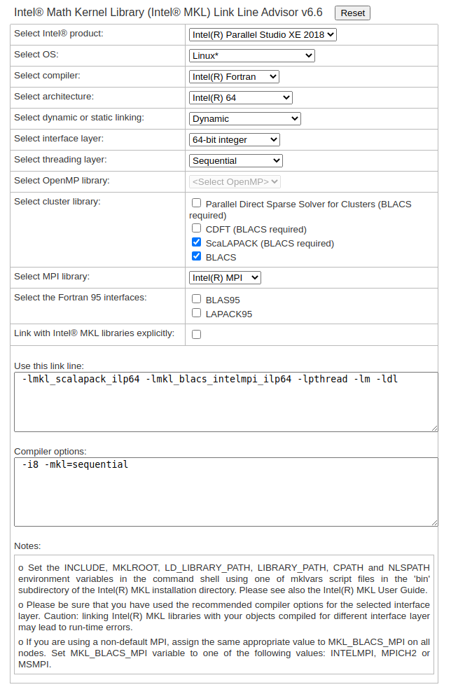
The compiler options and the link lines are then used build your application with ScaLAPACK.
Problems with the instructions on this section? Please send comments here.
Trilinos¶
“The Trilinos Project is a community of developers, users and user-developers focused on collaborative creation of algorithms and enabling technologies within an object-oriented software framework for the solution of large-scale, complex multi-physics engineering and scientific problems on new and emerging high-performance computing (HPC) architectures.” –Trilinos website
Trilinos now contains more than 50 packages. Most users use only a subset of them. It is recommended to make a customized build under your home or group directory. The Hoffman2 support group has expertise in using Trilinos. Please contact Technical support if you have Hoffman2-specific Trilinos questions.
Problems with the instructions on this section? Please send comments here.
zlib¶
“zlib is designed to be a free, general-purpose, legally unencumbered – that is, not covered by any patents – lossless data-compression library for use on virtually any computer hardware and operating system. The zlib data format is itself portable across platforms.” –zlib website
Request an interactive session with the needed resources (e.g., run-time, memory, number of cores, etc.), for example with:
$ qrsh -l h_data=2G,h_rt=1:00:00
To load the default version of zlib into your environment, use the command:
$ module load zlib
Once loaded, zlib’s top level, include file, and
library directories are defined by the environment variables
ZLIB_DIR, $ZLIB_INC and $ZLIB_LIB, respectively, which
can be used to compile and link your program.
Use the following command to discover other zlib versions:
$ module available zlib
See Environmental modules for further information.
Problems with the instructions on this section? Please send comments here.
Bioinformatics and biostatistics¶
Affymetrix - Analysis Power Tools¶
“The Analysis Power Tools (APT) is a collection of command line programs for analyzing and working with Affymetrix microarray data. These programs are generally focused on CEL file level analysis.” – Affymetrix APT Documentation
After requesting an interactive session with the needed resources (e.g., run-time, memory, number of cores, etc.), for example with:
$ qrsh -l h_data=2G,h_rt=1:00:00
You can check the available versions of Affymetrics’ Analysis Power Tools with:
$ module av affymetrix
To load the default version of the Affymetrix Analysis Power Tools, issue:
$ module load affymetrix
You can load a different version of Affymetrix Analysis Power Tools in your environment with:
$ module load affymetrix/VERSION
where VERSION is replaced by the desired version of affymetrix.
To get the help menu of apt-probeset-summarize:
$ apt-probeset-summarize --help
To see which Affymetrics’ Analysis Power Tools are available, please refer to the Affymetrics’ Analysis Power Tools documentation.
To submit a job for batch execution which uses any of the Affymetrics’ Analysis Power Tools you will need to create a submission script similar to:
### submit_job.sh START ###
#!/bin/bash
#$ -cwd
# error = Merged with joblog
#$ -o joblog.$JOB_ID
#$ -j y
# Edit the line starting with "#$ -l" to request the appropriate runtime and memory
# (or to add any other resource) as needed:
#$ -l h_rt=1:00:00,h_data=1G
# Add multiple cores/nodes as needed (also edit the parallel environment if needed):
#$ -pe shared 1
# Email address to notify
#$ -M $USER@mail
# Notify when
#$ -m bea

# echo job info on joblog:
echo "Job $JOB_ID started on:   " `hostname -s`
echo "Job $JOB_ID started on:   " `date `
echo " "

# load the job environment:
. /u/local/Modules/default/init/modules.sh
module load affymetrics

# substitute the command to run the needed APT command below:
echo 'apt-probeset-summarize -a rma-sketch -a plier-mm-sketch -d chip.cdf -o output-dir *.cel'
apt-probeset-summarize -a rma-sketch -a plier-mm-sketch -d chip.cdf -o output-dir *.cel

# echo job info on joblog:
echo "Job $JOB_ID ended on:   " `hostname -s`
echo "Job $JOB_ID ended on:   " `date `
echo " "
### submit_job.sh STOP ###
where you would replace the resources requested and the APT command as needed. Save the APT_submit.sh script in a location on your account from which you would like to submit your job, mark the script as an executable script with:
$ chmod u+x submit_job.sh
Submit the job with:
$ qsub APT_submit.sh
Problems with the instructions on this section? Please send comments here.
ANNOVAR¶
“ANNOVAR is an efficient software tool to utilize update-to-date information to functionally annotate genetic variants detected from diverse genomes (including human genome hg18, hg19, hg38, as well as mouse, worm, fly, yeast and many others).” – ANNOVAR Documentation
Running ANNOVAR to prepare local annotation databases
Preparation of local annotation databases using ANNOVAR requires downloading databases from outside of the Hoffman2 cluster. This step should be performed from the Hoffman2 transfer node (referred to as dtn). The transfer node can be accessed from your local computer via terminal and an ssh client:
$ ssh login_id@dtn.hoffman2.idre.ucla.edu
or, from any node of Hoffman2, with either:
$ ssh dtn1
or:
$ ssh dtn2
From the transfer node load ANNOVAR in your environment:
$ module load annovar
and use the ANNOVAR command to prepare a local annotation database:
$ annotate_variation.pl -downdb [optional arguments] <table-name> <output-directory-name>
After requesting an interactive session with the needed resources (e.g., run-time, memory, number of cores, etc.), for example with:
$ qrsh -l h_data=2G,h_rt=1:00:00
you can check the available versions of ANNOVAR with:
$ module av annovar
To load the default version of ANNOVAR, issue:
$ module load annovar
You can load a different version of ANNOVAR in your environment with:
$ module load annovar/VERSION
where VERSION is replaced by the desired version of ANNOVAR.
To use ANNOVAR, invoke any of the needed perl script from within the interactive session. For example, to invoke table_annovar.pl, issue:
$ table_annovar.pl --help
To submit a job for batch execution with ANNOVAR, you will need to create a submission script similar to:
### ANNOVAR_submit.sh START ###
#!/bin/bash
#$ -cwd
# error = Merged with joblog
#$ -o joblog.$JOB_ID
#$ -j y
# Edit the line below to request the appropriate runtime and memory
# (or to add any other resource) as needed:
#$ -l h_rt=1:00:00,h_data=1G
# Add multiple cores/nodes as needed:
#$ -pe shared 1
# Email address to notify
#$ -M $USER@mail
# Notify when
#$ -m bea

# echo job info on joblog:
echo "Job $JOB_ID started on:   " `hostname -s`
echo "Job $JOB_ID started on:   " `date `
echo " "

# load the job environment:
. /u/local/Modules/default/init/modules.sh
module load annovar

# in the following two lines substitute the command with the
# needed ANNOVAR command below:
echo "annotate_variation.pl --help"
annotate_variation.pl --help


# echo job info on joblog:
echo "Job $JOB_ID ended on:   " `hostname -s`
echo "Job $JOB_ID ended on:   " `date `
echo " "
### ANNOVAR_submit.sh STOP ###
where you would replace the resources requested and the ANNOVAR command as needed. Save the ANNOVAR_submit.sh script in a location on your account from which you would like to submit your job. Mark the script as an executable script with:
$ chmod u+x ANNOVAR_submit.sh
Submit the job with:
$ qsub ANNOVAR_submit.sh
Problems with the instructions on this section? Please send comments here.
BAMTools¶
“A software suite for programmers and end users that facilitates research analysis and data management using BAM files. BamTools provides both the first C++ API publicly available for BAM file support as well as a command-line toolkit.” – BAMTools
After requesting an interactive session (remember to specify a runtime, memory, number of computational cores, etc. as needed), for example with:
$ qrsh -l h_rt=1:00:00,h_data=2G -pe shared 2
you can check the available versions of BAMTools with:
$ module av bamtools
Load the default version of BAMTools in your environment with:
$ module load bamtools
To load a different version, issue:
$ module load bamtools/VERSION
where VERSION is replaced by the desired version of BAMTools.
To invoke BAMTools, enter:
$ bamtools &
Please refer to the BAMTools documentation to learn how to use this software.
To submit a job for batch execution with BAMTools, you will need to create a submission script similar to:
### bamtools_submit.sh START ###
#!/bin/bash
#$ -cwd
# error = Merged with joblog
#$ -o joblog.$JOB_ID
#$ -j y
# Edit the line below to request the appropriate runtime and memory
# (or to add any other resource) as needed:
#$ -l h_rt=1:00:00,h_data=1G
# Add multiple cores/nodes as needed:
#$ -pe shared 1
# Email address to notify
#$ -M $USER@mail
# Notify when
#$ -m bea

# echo job info on joblog:
echo "Job $JOB_ID started on:   " `hostname -s`
echo "Job $JOB_ID started on:   " `date `
echo " "

# load the job environment:
. /u/local/Modules/default/init/modules.sh
module load bamtools

# substitute the command to run the needed BAMTools command below:
echo '$SAMPLECOMMAND'
$SAMPLECOMMAND

# echo job info on joblog:
echo "Job $JOB_ID ended on:   " `hostname -s`
echo "Job $JOB_ID ended on:   " `date `
echo " "
### bamtools_submit.sh STOP ###
where you would replace the resources requested and the BAMTools command as needed. Save the BAMTools_submit.sh script in a location on your account from which you would like to submit your job, mark the script as an executable script with:
$ chmod u+x bamtools_submit.sh
Submit the job with:
$ qsub bamtools_submit.sh
Problems with the instructions on this section? Please send comments here.
BEDtools¶
“The BEDTools allow a fast and flexible way of comparing large datasets of genomic features. The BEDtools utilities allow one to address common genomics tasks such as finding feature overlaps and computing coverage.” – BEDtools
After requesting an interactive session (remember to specify a runtime, memory, number of computational cores, etc. as needed), for example with:
$ qrsh -l h_rt=1:00:00,h_data=2G -pe shared 2
you can check the available versions of BEDtools with:
$ module av bedtools
Load the default version of BEDtools in your environment with:
$ module load bedtools
To load a different version, issue:
$ module load bedtools/VERSION
where VERSION is replaced by the desired version of BEDtools.
To invoke BEDtools:
$ bedtools &
Please refer to BEDtools documentation to learn how to use this software BEDtools documentation.
To submit a job for batch execution with BEDtools, you will need to create a submission script similar to:
### BEDtools_submit.sh START ###
#!/bin/bash
#$ -cwd
# error = Merged with joblog
#$ -o joblog.$JOB_ID
#$ -j y
# Edit the line below to request the appropriate runtime and memory
# (or to add any other resource) as needed:
#$ -l h_rt=1:00:00,h_data=1G
# Add multiple cores/nodes as needed:
#$ -pe shared 1
# Email address to notify
#$ -M $USER@mail
# Notify when
#$ -m bea

# echo job info on joblog:
echo "Job $JOB_ID started on:   " `hostname -s`
echo "Job $JOB_ID started on:   " `date `
echo " "

# load the job environment:
. /u/local/Modules/default/init/modules.sh
module load bedtools

# substitute the command to run the needed BEDtools command below:
echo '$SAMPLECOMMAND'
$SAMPLECOMMAND

# echo job info on joblog:
echo "Job $JOB_ID ended on:   " `hostname -s`
echo "Job $JOB_ID ended on:   " `date `
echo " "
### BEDtools_submit.sh STOP ###
where you would replace the resources requested and the BEDtools command as needed. Save the BEDtools_submit.sh script in a location on your account from which you would like to submit your job. Mark the script as an executable script with:
$ chmod u+x BEDtools_submit.sh
Submit the job with:
$ qsub BEDtools_submit.sh
Problems with the instructions on this section? Please send comments here.
Bowtie¶
“An ultrafast memory-efficient short read aligner. Bowtie helps you visualize your data interactively. No javascript required, you build your dashboard in pure Python. Easy to deploy so you can share results with others.” – Bowtie
After requesting an interactive session (remember to specify a runtime, memory, number of computational cores, etc. as needed), for example with:
$ qrsh -l h_rt=1:00:00,h_data=2G -pe shared 2
you can check the available versions of Bowtie with:
$ module av bowtie
Load the default version of Bowtie in your environment with:
$ module load bowtie
To load a different version, issue:
$ module load bowtie/VERSION
where VERSION is replaced by the desired version of Bowtie.
To invoke bowtie:
$ bowtie &
Please refer to Bowtie documentation to learn how to use this software.
To submit a job for batch execution with Bowtie, you will need to create a submission script similar to:
### Bowtie_submit.sh START ###
#!/bin/bash
#$ -cwd
# error = Merged with joblog
#$ -o joblog.$JOB_ID
#$ -j y
# Edit the line below to request the appropriate runtime and memory
# (or to add any other resource) as needed:
#$ -l h_rt=1:00:00,h_data=1G
# Add multiple cores/nodes as needed:
#$ -pe shared 1
# Email address to notify
#$ -M $USER@mail
# Notify when
#$ -m bea

# echo job info on joblog:
echo "Job $JOB_ID started on:   " `hostname -s`
echo "Job $JOB_ID started on:   " `date `
echo " "

# load the job environment:
. /u/local/Modules/default/init/modules.sh
module load bowtie

# substitute the command to run the needed Bowtie command below:
echo '$SAMPLECOMMAND'
$SAMPLECOMMAND

# echo job info on joblog:
echo "Job $JOB_ID ended on:   " `hostname -s`
echo "Job $JOB_ID ended on:   " `date `
echo " "
### Bowtie_submit.sh STOP ###
where you would replace the resources requested and the Bowtie command as needed. Save the Bowtie_submit.sh script in a location on your account from which you would like to submit your job. Mark the script as an executable script with:
$ chmod u+x Bowtie_submit.sh
Submit the job with:
$ qsub Bowtie_submit.sh
Problems with the instructions on this section? Please send comments here.
BWA¶
“Burrows-Wheeler Aligner, BWA, is a software package for mapping low-divergent sequences against a large reference genome.” – BWA
After requesting an interactive session (remember to specify a runtime, memory, number of computational cores, etc. as needed), for example with:
$ qrsh -l h_rt=1:00:00,h_data=2G -pe shared 2
you can check the available versions of BWA with:
$ module av bwa
Load the default version of BWA in your environment with:
$ module load bwa
To load a different version, issue:
$ module load bwa/VERSION
where VERSION is replaced by the desired version of BWA.
To invoke BWA, enter:
$ bwa &
Please refer to the BWA documentation to learn how to use this software.
To submit a job for batch execution with BWA, you will need to create a submission script similar to:
### BWA_submit.sh START ###
#!/bin/bash
#$ -cwd
# error = Merged with joblog
#$ -o joblog.$JOB_ID
#$ -j y
# Edit the line below to request the appropriate runtime and memory
# (or to add any other resource) as needed:
#$ -l h_rt=1:00:00,h_data=1G
# Add multiple cores/nodes as needed:
#$ -pe shared 1
# Email address to notify
#$ -M $USER@mail
# Notify when
#$ -m bea

# echo job info on joblog:
echo "Job $JOB_ID started on:   " `hostname -s`
echo "Job $JOB_ID started on:   " `date `
echo " "

# load the job environment:
. /u/local/Modules/default/init/modules.sh
module load BWA

# substitute the command to run the needed BWA command below:
echo '$SAMPLECOMMAND'
$SAMPLECOMMAND

# echo job info on joblog:
echo "Job $JOB_ID ended on:   " `hostname -s`
echo "Job $JOB_ID ended on:   " `date `
echo " "
### BWA_submit.sh STOP ###
where you would replace the resources requested and the BWA command as needed. Save the BWA_submit.sh script in a location on your account from which you would like to submit your job. Mark the script as an executable script with:
$ chmod u+x BWA_submit.sh
Submit the job with:
$ qsub BWA_submit.sh
Problems with the instructions on this section? Please send comments here.
Cellranger¶
Under construction…
Cufflinks¶
“Cufflinks assembles transcripts, estimates their abundances, and tests for differential expression and regulation in RNA-Seq samples. It accepts aligned RNA-Seq reads and assembles the alignments into a parsimonious set of transcripts. Cufflinks then estimates the relative abundances of these transcripts based on how many reads support each one, taking into account biases in library preparation protocols.” – Cufflinks
After requesting an interactive session (remember to specify a runtime, memory, number of computational cores, etc. as needed), for example with:
$ qrsh -l h_rt=1:00:00,h_data=2G -pe shared 2
you can check the available versions of Cufflinks with:
$ module av cufflinks
Load the default version of Cufflinks in your environment with:
$ module load cufflinks
To load a different version, issue:
$ module load cufflinks/VERSION
where VERSION is replaced by the desired version of Cufflinks.
To invoke Cufflinks:
$ cufflinks &
Please refer to the Cufflinks documentation to learn how to use this software.
To submit a job for batch execution with Cufflinks, you will need to create a submission script similar to:
### Cufflinks_submit.sh START ###
#!/bin/bash
#$ -cwd
# error = Merged with joblog
#$ -o joblog.$JOB_ID
#$ -j y
# Edit the line below to request the appropriate runtime and memory
# (or to add any other resource) as needed:
#$ -l h_rt=1:00:00,h_data=1G
# Add multiple cores/nodes as needed:
#$ -pe shared 1
# Email address to notify
#$ -M $USER@mail
# Notify when
#$ -m bea

# echo job info on joblog:
echo "Job $JOB_ID started on:   " `hostname -s`
echo "Job $JOB_ID started on:   " `date `
echo " "

# load the job environment:
. /u/local/Modules/default/init/modules.sh
module load Cufflinks

# substitute the command to run the needed Cufflinks command below:
echo '$SAMPLECOMMAND'
$SAMPLECOMMAND

# echo job info on joblog:
echo "Job $JOB_ID ended on:   " `hostname -s`
echo "Job $JOB_ID ended on:   " `date `
echo " "
### Cufflinks_submit.sh STOP ###
where you would replace the resources requested and the Cufflinks command as needed. Save the Cufflinks_submit.sh script in a location on your account from which you would like to submit your job. Mark the script as an executable script with:
$ chmod u+x Cufflinks_submit.sh
Submit the job with:
$ qsub Cufflinks_submit.sh
Problems with the instructions on this section? Please send comments here.
Galaxy¶
“Galaxy is an open source, web-based platform for data intensive biomedical research.” –Galaxy website
If you are interested in using the Galaxy server on the Hoffman2 Cluster, please contact Weihong Yan wyan@chem.ucla.edu for authorization.
Problems with the instructions on this section? Please send comments here.
GATK¶
“The Genome Analysis Toolkit (GATK) is a set of bioinformatic tools for analyzing high-throughput sequencing (HTS) and variant call format (VCF) data. The toolkit is well established for germline short variant discovery from whole genome and exome sequencing data. GATK4 expands functionality into copy number and somatic analyses and offers pipeline scripts for workflows. Version 4 (GATK4) is open-source at https://github.com/broadinstitute/gatk.” – GATK
After requesting an interactive session (remember to specify a runtime, memory, number of computational cores, etc. as needed), for example with:
$ qrsh -l h_rt=1:00:00,h_data=2G -pe shared 2
you can check the available versions of GATK with:
$ module av gatk
Load the default version of GATK in your environment with:
$ module load gatk
To load a different version, issue:
$ module load gatk/VERSION
where VERSION is replaced by the desired version of GATK.
To invoke GATK, enter:
$ gatk &
Please refer to the GATK documentation to learn how to use this software.
To submit a job for batch execution with GATK, you will need to create a submission script similar to:
### gatk_submit.sh START ###
#!/bin/bash
#$ -cwd
# error = Merged with joblog
#$ -o joblog.$JOB_ID
#$ -j y
# Edit the line below to request the appropriate runtime and memory
# (or to add any other resource) as needed:
#$ -l h_rt=1:00:00,h_data=1G
# Add multiple cores/nodes as needed:
#$ -pe shared 1
# Email address to notify
#$ -M $USER@mail
# Notify when
#$ -m bea

# echo job info on joblog:
echo "Job $JOB_ID started on:   " `hostname -s`
echo "Job $JOB_ID started on:   " `date `
echo " "

# load the job environment:
. /u/local/Modules/default/init/modules.sh
module load gatk

# substitute the command to run the needed gatk command below:
echo '$SAMPLECOMMAND'
$SAMPLECOMMAND

# echo job info on joblog:
echo "Job $JOB_ID ended on:   " `hostname -s`
echo "Job $JOB_ID ended on:   " `date `
echo " "
### gatk_submit.sh STOP ###
where you would replace the resources requested and the gatk command as needed. Save the gatk_submit.sh script in a location on your account from which you would like to submit your job. Mark the script as an executable script with:
$ chmod u+x gatk_submit.sh
Submit the job with:
$ qsub gatk_submit.sh
Problems with the instructions on this section? Please send comments here.
IMPUTE2¶
“IMPUTE version 2 (also known as IMPUTE2) is a genotype imputation and haplotype phasing program based on ideas from Howie et al. 2009:
Howie, P. Donnelly, and J. Marchini (2009) A flexible and accurate genotype imputation method for the next generation of genome-wide association studies. PLoS Genetics 5(6): e1000529 [Open Access Article] [Supplementary Material]”
– IMPUTE 2 documentation website
After requesting an interactive session (remember to specify a runtime, memory, number of computational cores, etc. as needed), for example with:
$ qrsh -l h_rt=1:00:00,h_data=2G -pe shared 2
you can check the available versions of IMPUTE with:
$ module av impute
Load the default version of IMPUTE in your environment with:
$ module load impute
To load a different version, issue:
$ module load impute/VERSION
where VERSION is replaced by the desired version of IMPUTE.
To invoke IMPUTE:
$ impute &
Please refer to the IMPUTE documentation to learn how to use this software.
To submit a job for batch execution with IMPUTE, you will need to create a submission script similar to:
### impute_submit.sh START ###
#!/bin/bash
#$ -cwd
# error = Merged with joblog
#$ -o joblog.$JOB_ID
#$ -j y
# Edit the line below to request the appropriate runtime and memory
# (or to add any other resource) as needed:
#$ -l h_rt=1:00:00,h_data=1G
# Add multiple cores/nodes as needed:
#$ -pe shared 1
# Email address to notify
#$ -M $USER@mail
# Notify when
#$ -m bea

# echo job info on joblog:
echo "Job $JOB_ID started on:   " `hostname -s`
echo "Job $JOB_ID started on:   " `date `
echo " "

# load the job environment:
. /u/local/Modules/default/init/modules.sh
module load impute

# substitute the command to run the needed impute command below:
echo '$SAMPLECOMMAND'
$SAMPLECOMMAND

# echo job info on joblog:
echo "Job $JOB_ID ended on:   " `hostname -s`
echo "Job $JOB_ID ended on:   " `date `
echo " "
### impute_submit.sh STOP ###
where you would replace the resources requested and the IMPUTE command as needed. Save the impute_submit.sh script in a location on your account from which you would like to submit your job. Mark the script as an executable script with:
$ chmod u+x impute_submit.sh
Submit the job with:
$ qsub impute_submit.sh
Problems with the instructions on this section? Please send comments here.
InsPecT¶
“A Computational Tool to Infer mRNA Synthesis, Processing and Degradation Dynamics From RNA- And 4sU-seq Time Course Experiments” – Inspect
Warning
Inspect is currently not loaded on Hoffman2 Cluster.
After requesting an interactive session (remember to specify a runtime, memory, number of computational cores, etc. as needed), for example with:
$ qrsh -l h_rt=1:00:00,h_data=2G -pe shared 2
you can check the available versions of Inspect with:
$ module av inspect
Load the default version of Inspect in your environment with:
$ module load inspect
To load a different version, issue:
$ module load inspect/VERSION
where VERSION is replaced by the desired version of Inspect.
To invoke Inspect:
$ inspect &
Please refer to the Inspect documentation to learn how to use this software.
To submit a job for batch execution with Inspect, you will need to create a submission script similar to:
### Inspect_submit.sh START ###
#!/bin/bash
#$ -cwd
# error = Merged with joblog
#$ -o joblog.$JOB_ID
#$ -j y
# Edit the line below to request the appropriate runtime and memory
# (or to add any other resource) as needed:
#$ -l h_rt=1:00:00,h_data=1G
# Add multiple cores/nodes as needed:
#$ -pe shared 1
# Email address to notify
#$ -M $USER@mail
# Notify when
#$ -m bea

# echo job info on joblog:
echo "Job $JOB_ID started on:   " `hostname -s`
echo "Job $JOB_ID started on:   " `date `
echo " "

# load the job environment:
. /u/local/Modules/default/init/modules.sh
module load Inspect

# substitute the command to run the needed Inspect command below:
echo '$SAMPLECOMMAND'
$SAMPLECOMMAND

# echo job info on joblog:
echo "Job $JOB_ID ended on:   " `hostname -s`
echo "Job $JOB_ID ended on:   " `date `
echo " "
### Inspect_submit.sh STOP ###
where you would replace the resources requested and the Inspect command as needed. Save the Inspect_submit.sh script in a location on your account from which you would like to submit your job. Mark the script as an executable script with:
$ chmod u+x inspect_submit.sh
Submit the job with:
$ qsub Inspect_submit.sh
Problems with the instructions on this section? Please send comments here.
MAQ¶
“Maq is a software that builds mapping assemblies from short reads generated by the next-generation sequencing machines. It is particularly designed for Illumina-Solexa 1G Genetic Analyzer, and has a preliminary functionality to handle AB SOLiD data.” – maq
After requesting an interactive session (remember to specify a runtime, memory, number of computational cores, etc. as needed), for example with:
$ qrsh -l h_rt=1:00:00,h_data=2G -pe shared 2
you can check the available versions of Maq with:
$ module av maq
Load the default version of maq in your environment with:
$ module load maq
To load a different version, issue:
$ module load maq/VERSION
where VERSION is replaced by the desired version of Maq.
To invoke maq:
$ maq &
Please refer to the Maq documentation to learn how to use this software.
To submit a job for batch execution with Maq, you will need to create a submission script similar to:
### maq_submit.sh START ###
#!/bin/bash
#$ -cwd
# error = Merged with joblog
#$ -o joblog.$JOB_ID
#$ -j y
# Edit the line below to request the appropriate runtime and memory
# (or to add any other resource) as needed:
#$ -l h_rt=1:00:00,h_data=1G
# Add multiple cores/nodes as needed:
#$ -pe shared 1
# Email address to notify
#$ -M $USER@mail
# Notify when
#$ -m bea

# echo job info on joblog:
echo "Job $JOB_ID started on:   " `hostname -s`
echo "Job $JOB_ID started on:   " `date `
echo " "

# load the job environment:
. /u/local/Modules/default/init/modules.sh
module load maq

# substitute the command to run the needed maq command below:
echo '$SAMPLECOMMAND'
$SAMPLECOMMAND

# echo job info on joblog:
echo "Job $JOB_ID ended on:   " `hostname -s`
echo "Job $JOB_ID ended on:   " `date `
echo " "
### maq_submit.sh STOP ###
where you would replace the resources requested and the Maq command as needed. Save the maq_submit.sh script in a location on your account from which you would like to submit your job. Mark the script as an executable script with:
$ chmod u+x maq_submit.sh
Submit the job with:
$ qsub maq_submit.sh
Problems with the instructions on this section? Please send comments here.
Picard Tools¶
“Picard is a set of command line tools for manipulating high-throughput sequencing (HTS) data and formats such as SAM/BAM/CRAM and VCF” – Picard Tools
After requesting an interactive session (remember to specify a runtime, memory, number of computational cores, etc. as needed), for example with:
$ qrsh -l h_rt=1:00:00,h_data=4G -pe shared 1
you can check the available versions of Picard Tools with:
$ module av picard_tools
Load the default version of Picard Tools in your environment with:
$ module load picard_tools
To load a different version, if available, issue:
$ module load picard_tools/VERSION
where VERSION is replaced by the desired version of Picard Tools.
To run Picard Tools at the shell prompt issue:
$ java [jvm-args] -jar $PICARD <PicardToolName> [OPTION1=value1] [OPTION2=value2] [...]
where:
<PicardToolName>is one of the tools available in the Picard toolkit[OPTION1=value1]key-value pairs are standard options relative to the particular<PicardToolName>[jvm-args]are java arguments (most of the commands are designed to run in 2GB of JVM, so it is recommended using the JVM argument-Xmx2g)
To see a list of available <PicardToolName> you can issue:
$ java -jar $PICARD -h
to see a list of options (i.e., [OPTION1=value1]) for each <PicardToolName> you can issue:
$ java -jar $PICARD <PicardToolName> -h
to see a full list of java options issue:
$ java -h
and to see the list of java options issue:
$ java -X
Please refer to the Picard Tools documentation to learn how to use this software.
To submit a job for batch execution with Picard Tools, you will need to create a submission script similar to:
### picard_tools_submit.sh START ###
#!/bin/bash
#$ -cwd
# error = Merged with joblog
#$ -o joblog.$JOB_ID
#$ -j y
# Edit the line below to request the appropriate runtime and memory
# (or to add any other resource) as needed:
#$ -l h_rt=1:00:00,h_data=2G
# Add multiple cores/nodes as needed:
#$ -pe shared 1
# Email address to notify
#$ -M $USER@mail
# Notify when
#$ -m bea

# echo job info on joblog:
echo "Job $JOB_ID started on:   " `hostname -s`
echo "Job $JOB_ID started on:   " `date `
echo " "

# load the job environment:
. /u/local/Modules/default/init/modules.sh
module load picard_tools

# substitute the command to run the needed Picard Tools command below:
echo 'java [jvm-args] -jar $PICARD <PicardToolName> [OPTION1=value1] [OPTION2=value2] [...]'
java [jvm-args] -jar $PICARD <PicardToolName> [OPTION1=value1] [OPTION2=value2] [...]

# echo job info on joblog:
echo "Job $JOB_ID ended on:   " `hostname -s`
echo "Job $JOB_ID ended on:   " `date `
echo " "
### picard_tools_submit.sh STOP ###
where you would replace the resources requested (-l h_rt=1:00:00,h_data=2G and -pe shared 1) and the Picard Tools command (java [jvm-args] -jar $PICARD ...) as needed. Save the picard_tools_submit.sh script in a location on your account from which you would like to submit your job. Mark the script as an executable script with:
$ chmod u+x picard_tools_submit.sh
submit the job with:
$ qsub picard_tools_submit.sh
Problems with the instructions on this section? Please send comments here.
PLINK¶
“PLINK is a free, open-source whole genome association analysis toolset, designed to perform a range of basic, large-scale analyses in a computationally efficient manner.” – PLINK
After requesting an interactive session (remember to specify a runtime, memory, number of computational cores, etc. as needed), for example with:
$ qrsh -l h_rt=1:00:00,h_data=2G -pe shared 2
you can check the available versions of PLINK with:
$ module av plink
Load the default version of PLINK in your environment with:
$ module load plink
To load a different version, issue:
$ module load plink/VERSION
where VERSION is replaced by the desired version of PLINK.
To invoke PLINK:
$ plink &
Enter the PLINK command with any arguments. For example:
$ plink -ped test.ped --map test.map --maf 0.05 --assoc
where test.ped and test.map are your ped and map files.
$ java -jar /u/local/apps/plink/1.06/gPLINK2.jar
To run PLINK Interactively with R and Rserve, click R-plugins for details and examples.
If you need to use the functionalities of the statistical package R with PLINK, first use qrsh to obtain an interactive compute node, and load PLINK into your environment.
$ Start Rserve
$ module load R
$ R CMD Rserve
Rserve will run daemonized as a server. Verify it is running with
$ ps aux | grep Rserve
Please remember to kill the Rserve process when is no longer needed. Get the process ID from the command ps aux | grep Rserve and then enter kill pid where pid is the process ID.
To change the directory where your data to be analyzed is located, enter:
$ cd mydir
Enter the PLINK command with any arguments:
$ plink arguments
After you finish, kill the Rserve daemon on the same node where you started it before you exit your qrsh session. To do so, enter:
$ ps aux | grep Rserve
$ kill pid
where pid is the process ID of your Rserve process.
Please refer to the PLINK documentation to learn how to use this software.
To submit a job for batch execution with PLINK, you will need to create a submission script similar to:
### plink_submit.sh START ###
#!/bin/bash
#$ -cwd
# error = Merged with joblog
#$ -o joblog.$JOB_ID
#$ -j y
# Edit the line below to request the appropriate runtime and memory
# (or to add any other resource) as needed:
#$ -l h_rt=1:00:00,h_data=1G
# Add multiple cores/nodes as needed:
#$ -pe shared 1
# Email address to notify
#$ -M $USER@mail
# Notify when
#$ -m bea

# echo job info on joblog:
echo "Job $JOB_ID started on:   " `hostname -s`
echo "Job $JOB_ID started on:   " `date `
echo " "

# load the job environment:
. /u/local/Modules/default/init/modules.sh
module load plink

# substitute the command to run the needed plink command below:
echo '$SAMPLECOMMAND'
$SAMPLECOMMAND

# echo job info on joblog:
echo "Job $JOB_ID ended on:   " `hostname -s`
echo "Job $JOB_ID ended on:   " `date `
echo " "
### plink_submit.sh STOP ###
where you would replace the resources requested and the PLINK command as needed. Save the plink_submit.sh script in a location on your account from which you would like to submit your job. Mark the script as an executable script with:
$ chmod u+x plink_submit.sh
Submit the job with:
$ qsub plink_submit.sh
Problems with the instructions on this section? Please send comments here.
SAMtools¶
“SAM (Sequence Alignment/Map) is a flexible generic format for storing nucleotide sequence alignment. SAM tools provide efficient utilities for manipulating alignments in the SAM and Bam formats.” – SAMtools
After requesting an interactive session (remember to specify a runtime, memory, number of computational cores, etc. as needed), for example with:
$ qrsh -l h_rt=1:00:00,h_data=2G -pe shared 2
you can check the available versions of SAMtools with:
$ module av samtools
Load the default version of SAMtools in your environment with:
$ module load samtools
To load a different version, issue:
$ module load samtools/VERSION
where VERSION is replaced by the desired version of SAMtools.
To invoke SAMtools:
$ samtools &
Please refer to the SAMtools documentation to learn how to use this software.
To submit a job for batch execution with SAMtools you will need to create a submission script similar to:
### samtools_submit.sh START ###
#!/bin/bash
#$ -cwd
# error = Merged with joblog
#$ -o joblog.$JOB_ID
#$ -j y
# Edit the line below to request the appropriate runtime and memory
# (or to add any other resource) as needed:
#$ -l h_rt=1:00:00,h_data=1G
# Add multiple cores/nodes as needed:
#$ -pe shared 1
# Email address to notify
#$ -M $USER@mail
# Notify when
#$ -m bea

# echo job info on joblog:
echo "Job $JOB_ID started on:   " `hostname -s`
echo "Job $JOB_ID started on:   " `date `
echo " "

# load the job environment:
. /u/local/Modules/default/init/modules.sh
module load samtools

# substitute the command to run the needed SAMtools command below:
echo '$SAMPLECOMMAND'
$SAMPLECOMMAND

# echo job info on joblog:
echo "Job $JOB_ID ended on:   " `hostname -s`
echo "Job $JOB_ID ended on:   " `date `
echo " "
### SAMtools_submit.sh STOP ###
where you would replace the resources requested and the SAMtools command as needed. Save the SAMtools_submit.sh script in a location on your account from which you would like to submit your job. Mark the script as an executable script with:
$ chmod u+x samtools_submit.sh
Submit the job with:
$ qsub samtools_submit.sh
Problems with the instructions on this section? Please send comments here.
SOLAR¶
“SOLAR-Eclipse is an extensive, flexible software package for genetic variance components analysis, including linkage analysis, quantitative genetic analysis, SNP association analysis (QTN and QTLD), and covariate screening. Operations are included for calculation of marker-specific or multipoint identity-by-descent (IBD) matrices in pedigrees of arbitrary size and complexity, and for linkage analysis of multiple quantitative traits and/or discrete traits which may involve multiple loci (oligogenic analysis), dominance effects, household effects, and interactions. Additional features include functionality for mega and meta-genetic analyses where data from diverse cohorts can be pooled to improve statistical significance.” – SOLAR
After requesting an interactive session (remember to specify a runtime, memory, number of computational cores, etc. as needed), for example with:
$ qrsh -l h_rt=1:00:00,h_data=2G -pe shared 2
you can check the available versions of SOLAR with:
$ module av solar
Load the default version of SOLAR in your environment with:
$ module load solar
To load a different version, issue:
$ module load solar/VERSION
where VERSION is replaced by the desired version of SOLAR.
To invoke solar:
$ solar &
Please refer to the SOLAR documentation to learn how to use this software.
To submit a job for batch execution when running SOLAR, you will need to create a submission script similar to:
### solar_submit.sh START ###
#!/bin/bash
#$ -cwd
# error = Merged with joblog
#$ -o joblog.$JOB_ID
#$ -j y
# Edit the line below to request the appropriate runtime and memory
# (or to add any other resource) as needed:
#$ -l h_rt=1:00:00,h_data=1G
# Add multiple cores/nodes as needed:
#$ -pe shared 1
# Email address to notify
#$ -M $USER@mail
# Notify when
#$ -m bea

# echo job info on joblog:
echo "Job $JOB_ID started on:   " `hostname -s`
echo "Job $JOB_ID started on:   " `date `
echo " "

# load the job environment:
. /u/local/Modules/default/init/modules.sh
module load solar

# substitute the command to run the needed solar command below:
echo '$SAMPLECOMMAND'
$SAMPLECOMMAND

# echo job info on joblog:
echo "Job $JOB_ID ended on:   " `hostname -s`
echo "Job $JOB_ID ended on:   " `date `
echo " "
### solar_submit.sh STOP ###
where you would replace the resources requested and the solar command as needed. Save the solar_submit.sh script in a location on your account from which you would like to submit your job. Mark the script as an executable script with:
$ chmod u+x solar_submit.sh
submit the job with:
$ qsub solar_submit.sh
Problems with the instructions on this section? Please send comments here.
TopHat¶
“TopHat is a fast splice junction mapper for RNA-Seq reads. It aligns RNA-Seq reads to mammalian-sized genomes using the ultra high-throughput short read aligner Bowtie, and then analyzes the mapping results to identify splice junctions between exons.” – TopHat
After requesting an interactive session (remember to specify a runtime, memory, number of computational cores, etc. as needed), for example with:
$ qrsh -l h_rt=1:00:00,h_data=2G -pe shared 2
you can check the available versions of TopHat with:
$ module av tophat
Load the default version of TopHat in your environment with:
$ module load tophat
To load a different version, issue:
$ module load tophat/VERSION
where VERSION is replaced by the desired version of TopHat.
To invoke TopHat:
$ tophat &
Please refer to the TopHat documentation to learn how to use this software.
To submit a job for batch execution with TopHat, you will need to create a submission script similar to:
### tophat_submit.sh START ###
#!/bin/bash
#$ -cwd
# error = Merged with joblog
#$ -o joblog.$JOB_ID
#$ -j y
# Edit the line below to request the appropriate runtime and memory
# (or to add any other resource) as needed:
#$ -l h_rt=1:00:00,h_data=1G
# Add multiple cores/nodes as needed:
#$ -pe shared 1
# Email address to notify
#$ -M $USER@mail
# Notify when
#$ -m bea

# echo job info on joblog:
echo "Job $JOB_ID started on:   " `hostname -s`
echo "Job $JOB_ID started on:   " `date `
echo " "

# load the job environment:
. /u/local/Modules/default/init/modules.sh
module load tophat

# substitute the command to run the needed tophat command below:
echo '$SAMPLECOMMAND'
$SAMPLECOMMAND

# echo job info on joblog:
echo "Job $JOB_ID ended on:   " `hostname -s`
echo "Job $JOB_ID ended on:   " `date `
echo " "
### tophat_submit.sh STOP ###
where you would replace the resources requested and the TopHat command as needed. Save the tophat_submit.sh script in a location on your account from which you would like to submit your job. Mark the script as an executable script with:
$ chmod u+x tophat_submit.sh
Submit the job with:
$ qsub tophat_submit.sh
Problems with the instructions on this section? Please send comments here.
TreeMix¶
“TreeMix is a method for inferring the patterns of population splits and mixtures in the history of a set of populations.” – TreeMix
After requesting an interactive session (remember to specify a runtime, memory, number of computational cores, etc. as needed), for example with:
$ qrsh -l h_rt=1:00:00,h_data=2G -pe shared 2
you can check the available versions of TreeMix with:
$ module av treemix
Load the default version of TreeMix in your environment with:
$ module load treemix
To load a different version, issue:
$ module load treemix/VERSION
where VERSION is replaced by the desired version of TreeMix.
To invoke TreeMix:
$ treemix &
Please refer to the TreeMix documentation to learn how to use this software.
To submit a job for batch execution with TreeMix, you will need to create a submission script similar to:
### treemix_submit.sh START ###
#!/bin/bash
#$ -cwd
# error = Merged with joblog
#$ -o joblog.$JOB_ID
#$ -j y
# Edit the line below to request the appropriate runtime and memory
# (or to add any other resource) as needed:
#$ -l h_rt=1:00:00,h_data=1G
# Add multiple cores/nodes as needed:
#$ -pe shared 1
# Email address to notify
#$ -M $USER@mail
# Notify when
#$ -m bea

# echo job info on joblog:
echo "Job $JOB_ID started on:   " `hostname -s`
echo "Job $JOB_ID started on:   " `date `
echo " "

# load the job environment:
. /u/local/Modules/default/init/modules.sh
module load treemix

# substitute the command to run the needed TreeMix command below:
echo '$SAMPLECOMMAND'
$SAMPLECOMMAND

# echo job info on joblog:
echo "Job $JOB_ID ended on:   " `hostname -s`
echo "Job $JOB_ID ended on:   " `date `
echo " "
### treemix_submit.sh STOP ###
where you would replace the resources requested and the TreeMix command as needed. Save the treemix_submit.sh script in a location on your account from which you would like to submit your job. Mark the script as an executable script with:
$ chmod u+x treemix_submit.sh
Submit the job with:
$ qsub treemix_submit.sh
Problems with the instructions on this section? Please send comments here.
VEGAS¶
“Versatile Gene-based Association Study” – VEGAS
After requesting an interactive session (remember to specify a runtime, memory, number of computational cores, etc. as needed), for example with:
$ qrsh -l h_rt=1:00:00,h_data=2G -pe shared 2
you can check the available versions of VEGAS with:
$ module av vegas
Load the default version of VEGAS in your environment with:
$ module load vegas
To load a different version, issue:
$ module load vegas/VERSION
where VERSION is replaced by the desired version of VEGAS.
To invoke VEGAS:
$ vegas &
Please refer to VEGAS documentation to learn how to use this software.
To submit a job for batch execution with VEGAS, you will need to create a submission script similar to:
### VEGAS_submit.sh START ###
#!/bin/bash
#$ -cwd
# error = Merged with joblog
#$ -o joblog.$JOB_ID
#$ -j y
# Edit the line below to request the appropriate runtime and memory
# (or to add any other resource) as needed:
#$ -l h_rt=1:00:00,h_data=1G
# Add multiple cores/nodes as needed:
#$ -pe shared 1
# Email address to notify
#$ -M $USER@mail
# Notify when
#$ -m bea

# echo job info on joblog:
echo "Job $JOB_ID started on:   " `hostname -s`
echo "Job $JOB_ID started on:   " `date `
echo " "

# load the job environment:
. /u/local/Modules/default/init/modules.sh
module load VEGAS

# substitute the command to run the needed VEGAS command below:
echo '$SAMPLECOMMAND'
$SAMPLECOMMAND

# echo job info on joblog:
echo "Job $JOB_ID ended on:   " `hostname -s`
echo "Job $JOB_ID ended on:   " `date `
echo " "
### VEGAS_submit.sh STOP ###
where you would replace the resources requested and the VEGAS command as needed. Save the vegas_submit.sh script in a location on your account from which you would like to submit your job, mark the script as an executable script with:
$ chmod u+x vegas_submit.sh
Submit the job with:
$ qsub vegas_submit.sh
Problems with the instructions on this section? Please send comments here.
Chemistry and chemical engineering¶
Amber¶
“Amber is the collective name for a suite of programs that allow users to carry out molecular dynamics simulations, particularly on biomolecules.” – Amber
After requesting an interactive session (remember to specify a runtime, memory, number of computational cores, etc.), for example with:
$ qrsh -l h_rt=1:00:00,h_data=2G -pe shared 2
you can check the available versions of Amber with:
$ module av amber
Load the default version of Amber in your environment with:
$ module load amber
To load a different version, issue:
$ module load amber/VERSION
where VERSION is replaced by the desired version of Amber.
To invoke one of the Amber executable, e.g. to check the version of sander issue:
$ sander --version
Please refer to Amber documentation to learn how to use this software.
To submit a job for batch execution with Amber, you will need to create a submission script similar to (the example below is relative to runnign sander on a restart job for of a water box from run 33 to 34):
### amber_submit.sh START ###
#!/bin/bash
#$ -cwd
# error = Merged with joblog
#$ -o joblog.$JOB_ID
#$ -j y
# Edit the line below to request the appropriate runtime and memory
# (or to add any other resource) as needed:
#$ -l h_rt=1:00:00,h_data=1G
# Add multiple cores/nodes as needed:
#$ -pe dc* 30
# Email address to notify
#$ -M $USER@mail
# Notify when
#$ -m bea

# echo job info on joblog:
echo "Job $JOB_ID started on:   " `hostname -s`
echo "Job $JOB_ID started on:   " `date `
echo " "

# load the job environment:
. /u/local/Modules/default/init/modules.sh
module load amber

export AMBER_HOME=$AMBERHOME

# substitute the command to run the needed Amber command below:

/usr/bin/time -v `which mpirun` -n $NSLOTS $AMBERHOME/bin/sander -O \
                                -i ./prod.in \
                                -c ./prod-33.rec \
                                -p ./water864.parm7 \
                                                    \
                                                    \
                                                    \
                                                    \
                                   -o ./prod-34.out \
                                                    \
                                                    \
                                  -e ./prod-34.mden \
                                  -inf prod-34.info \
                                                    \
                                                    \
                                                    \
                                     -r prod-34.rec \
                                                    \
                                     -v prod-34.vel \
                                                    \
                                                    \
                                                    \
                                                    \
                                     -x prod-34.crd \
                                     >& amber.output.$JOB_ID


# echo job info on joblog:
echo "Job $JOB_ID ended on:   " `hostname -s`
echo "Job $JOB_ID ended on:   " `date `
echo " "
### Amber_submit.sh STOP ###
where you would replace the resources requested and the Amber command as needed. Save the amber_submit.sh script in a location on your account from which you would like to submit your job, mark the script as an executable script with:
$ chmod u+x amber_submit.sh
Submit the job with:
$ qsub amber_submit.sh
Please refer to Amber documentation to learn how to use this software.
Problems with the instructions on this section? Please send comments here.
CP2K¶
“CP2K is a quantum chemistry and solid state physics software package that can perform atomistic simulations of solid state, liquid, molecular, periodic, material, crystal, and biological systems.” – CP2K
After requesting an interactive session (remember to specify a runtime, memory, number of computational cores, etc.), for example with:
$ qrsh -l h_rt=1:00:00,h_data=2G -pe shared 2
you can check the available versions of CP2K with:
$ module av cp2k
Load the default version of CP2K in your environment with:
$ module load cp2k
To invoke CP2K:
$ cp2k.popt --version
Please refer to CP2K documentation to learn how to use this software.
To submit a job for batch execution which uses any of the CP2K you will need to create a submission script similar to:
### cp2k_submit.sh START ###
#!/bin/bash
#$ -cwd
# error = Merged with joblog
#$ -o joblog.$JOB_ID
#$ -j y
# Edit the line below to request the appropriate runtime and memory
# (or to add any other resource) as needed:
#$ -l h_rt=1:00:00,h_data=1G
# Add multiple cores/nodes as needed:
#$ -pe dc* 30
# Email address to notify
#$ -M $USER@mail
# Notify when
#$ -m bea

# echo job info on joblog:
echo "Job $JOB_ID started on:   " `hostname -s`
echo "Job $JOB_ID started on:   " `date `
echo " "

# load the job environment:
. /u/local/Modules/default/init/modules.sh
module load cp2k

# substitute the command to run the needed cp2k command below:
time -v `which mpirun` -np $NSLOTS \
cp2k.popt  CP2K.inp >& CP2K.output.$JOB_ID


# echo job info on joblog:
echo "Job $JOB_ID ended on:   " `hostname -s`
echo "Job $JOB_ID ended on:   " `date `
echo " "
### cp2k_submit.sh STOP ###
where you would replace the resources requested and the CP2K command as needed. Save the cp2k_submit.sh script in a location on your account from which you would like to submit your job, mark the script as an executable script with:
$ chmod u+x cp2k_submit.sh
Submit the job with:
$ qsub cp2k_submit.sh
Please refer to CP2K documentation to learn how to use this software.
Problems with the instructions on this section? Please send comments here.
CPMD¶
Coming soon
This section is under construction. Please call again soon!
Gaussian¶
“Gaussian is a general purpose computational chemistry software package initially released in 1970 by John Pople and his research group at Carnegie Mellon University as Gaussian 70.” – Gaussian
Important
By contractual agreement with Gaussian, Inc., only authorized members of the UCLA community can use Gaussian. To request to be authorized to use Gaussian on the Hoffman2 Cluster you will need to perform the following two these actions:
navigate to the SIM account management portal and in the search bar below Request resource for your account type gaussian and press the adjacent REQUESTME button
notify Qingyang Zhou, of the UCLA Department of Chemistry, that you have made the request to access Gaussian on the SIM account management portal, you will need to sign an agreement
NOTE: failure to notify Qingyang Zhou may result delay in your access to Gaussian.
GaussView can be used to prepare inputs or visualize outputs. While GaussView can also be used to submit on the local node Gaussian jobs, it is preferable to submit Gaussian batch jobs via a submission script as described in Batch use.
Please refer to Gaussian documentation to learn how to use this software.
To submit Gaussian as a batch job you will need a submission script, a sample is given below. Please refer to Gaussian documentation to learn how to use this software. Some general directions on values to use in the Route Section of your Gaussian input file are given here:
In order for Gaussian to make use of your job’s memory allocation, your input file may include a %Mem instruction for dynamic memory. The default value for %Mem is 256MB or 32MW (mega-words) per core.
The %Mem value should be less than the memory per core that you request for your job. We recommend, for example, for a job requesting 1024MB per core enter:
%Mem=800MB
For jobs requesting 4096 MB per core, enter:
%Mem=3800MB
Modify the default %Mem value only if needed. A value that is too large may decrease the job’s performance instead of improving it.
If using Gaussian across multiple cores on the same compute node make sure to modify the Route Section of your job so that the %nprocshared directive is set to the same number of cores that you will request via the scheduler directive -pe shared N, that is, if for example requesting 36 cores add to your Gaussian input Route Section the line:
%nprocshared=36
accordingly you will need to make sure that your submission script contains the line:
#$ -pe shared 36
or submit your script with the command:
$ qsub -pe shared 36 -N YOUR_GAUSSIAN_INPUT_FILE_NAME submit_gaussian.sh
where YOUR_GAUSSIAN_INPUT_FILE_NAME is the name of your Gaussian input file and submit_gaussian.sh is a submission script as the one given below:
### submit_gaussian.sh START ###
###################################################################################################
# THIS SCRIPT ASSUMES THAT YOU WILL SUBMIT IT AS FOLLOWS:
# qsub -N YOUR_GAUSSIAN_INPUT_FILE_NAME submit_gaussian.sh
# YOU CAN MODIFY RESOURCES BELOW OR MODIFY THEM AT SUBMISSION, E.G.:
# qsub -N YOUR_GAUSSIAN_INPUT_FILE_NAME -l h_data=8G,h_rt=24:00:00 -pe shared 8 submit_gaussian.sh
# MAKE SURE THAT YOUR INPUT FILE PROLOG HAS A LINE:
# %nprocshared=8
# WITH THE SAME (OR LESS) NUMBER OF CORES REQUESTED (I.E.: -pe shared 8)
#!/bin/bash
#$ -cwd
#$ -o $JOB_NAME.joblog.$JOB_ID
#$ -j y
#$ -M $USER@mail
#$ -m bea
# CHANGE THE RESOURCES BELOW AS NEEDED:
#$ -l h_data=5G,h_rt=2:00:00,arch=intel-[Eg][5o][l-]*
# CHANGE THE NUMBER OF CORES AS NEEDED:
#$ -pe shared 36
###################################################################################################

# YOU GENERALLY WILL NOT NEED TO MODIFY THE LINES BELOW:

# echo job info on joblog:
echo "Job $JOB_ID started on:   " `hostname -s`
echo "Job $JOB_ID started on:   " `date `
echo " "

# set job environment and GAUSS_SCRDIR variable
. /u/local/Modules/default/init/modules.sh
module load gaussian
export GAUSS_SCRDIR=$TMPDIR
# echo in joblog
module li
echo "GAUSS_SCRDIR=$GAUSS_SCRDIR"
echo " "

echo "/usr/bin/time -v $g16root/g16 < ${JOB_NAME%.*}.com > ${JOB_NAME%.*}.out"
/usr/bin/time -v $g16root/g16 < ${JOB_NAME%.*}.com > ${JOB_NAME%.*}.out

# echo job info on joblog:
echo "Job $JOB_ID ended on:   " `hostname -s`
echo "Job $JOB_ID ended on:   " `date `
echo " "
echo "Input file START:"
cat ${JOB_NAME%.*}.com
echo "END of input file"
echo " "
### submit_gaussian.sh STOP ###
where you would replace the resources requested and the Gaussian command as needed. Save the submit_gaussian.sh script in a location on your account from which you would like to submit your job, mark the script as an executable script with:
$ chmod u+x submit_gaussian.sh
Submit the job with:
$ qsub -N submit_gaussian.sh
For older versions of the software you can use:
$ # general submission
$ g09.q # or: gaussian09.q

$ # general serial submission
$ g09.q.serial # or: gaussian09.q.serial

$ #Runs on multiple cpus on a single node:
$ g09.q.multithread # or: gaussian09.q.multithread


$ #Runs on multiple cpus on multiple whole nodes:
$ g09.q.parallel # or: gaussian09.q.parallel
Note that if you are using g09.q.parallel, your input file should not contain %NProcShared or %LindaWorkers, or %NProc or %NProcLinda instructions specifying the number of processors to be used, or the nodes you job should run on. Your job will request any needed processors at runtime.
Please refer to Gaussian documentation to learn how to use this software.
Problems with the instructions on this section? Please send comments here.
GaussView¶
GaussView is a graphical user to Gaussian. GaussView
Important
By contractual agreement with Gaussian, Inc., only authorized members of the UCLA community can use Gaussian. To request to be authorized to use Gaussian on the Hoffman2 Cluster you will need to perform the following two these actions:
navigate to the SIM account management portal and in the search bar below Request resource for your account type gaussian and press the adjacent REQUESTME button
notify Qingyang Zhou, of the UCLA Department of Chemistry, that you have made the request to access Gaussian on the SIM account management portal, you will need to sign an agreement
NOTE: failure to notify Qingyang Zhou may result delay in your access to Gaussian.
Note
To open the graphical user interface (GUI) of GaussView, you will need to have connected to the Hoffman2 Cluster either via a remote desktop or via terminal and SSH having followed directions on how to open GUI applications. Under these conditions, GaussView will start in GUI mode by default.
The GaussView program will let you submit a com file to Gaussian. The com file may be one created by GaussView, or one you created with a text editor. When you close your GaussView session, any Gaussian process that is still running will be aborted. If your calculations need to run for an extended period of time, we recommend that you instead run Gaussian in batch.
After requesting an interactive session (remember to specify the needed runtime, memory, number of computational cores, etc.), for example with:
$ qrsh -l h_rt=1:00:00,h_data=2G -pe shared 2
you can check the available versions of GaussView with:
$ gaussview
Please refer to GaussiView documentation to learn how to use this software.
Problems with the instructions on this section? Please send comments here.
GROMACS¶
“GROMACS is a versatile package to perform molecular dynamics, i.e. simulate the Newtonian equations of motion for systems with hundreds to millions of particles.” – GROMACS
To run the molecular dynamics part (mdrun) of the GROMACS suite of programs, you are required to have previously generated an input file containing information about the topology, the structure and the parameters of your system. Such input file, which generally has a .tpr, a .tpb or a .tpa extension, is generated via the grompp part of GROMACS.
You can execute the pre- and post-processing GROMACS tasks within an interactive session, which you can request for example with (remember to specify a runtime, memory, number of computational cores, etc. as needed):
$ qrsh -l h_rt=1:00:00,h_data=2G -pe shared 2
To run pre- and post-processing parts of GROMACS (such as gmx pdb2gmx, gmx solvate, gmx grompp, etc.) you need to set GROMACS into your environment by loading the gromacs module file. You can check the available versions of GROMACS with:
$ module av gromacs
Load the default version of gromacs in your environment with:
$ module load gromacs
To load a different version, issue:
$ module load gromacs/VERSION
where VERSION is replaced by the desired version of gromacs.
To check the version of GROMACS:
$ gmx -version
Please refer to GROMACS documentation to learn how to use this software.
To submit a job for batch execution with GROMACS, you will need to create a submission script similar to (remember to substitute $SAMPLECOMMAND for something like: gmx_mpi mpdrun ...):
### gromacs_submit.sh START ###
#!/bin/bash
#$ -cwd
# error = Merged with joblog
#$ -o joblog.$JOB_ID
#$ -j y
# Edit the line below to request the appropriate runtime and memory
# (or to add any other resource) as needed:
#$ -l h_rt=1:00:00,h_data=1G
# Add multiple cores/nodes as needed:
#$ -pe shared 1
# Email address to notify
#$ -M $USER@mail
# Notify when
#$ -m bea

# echo job info on joblog:
echo "Job $JOB_ID started on:   " `hostname -s`
echo "Job $JOB_ID started on:   " `date `
echo " "

# load the job environment:
. /u/local/Modules/default/init/modules.sh
module load gromacs

# substitute the command to run the needed gromacs command below:
echo '$SAMPLECOMMAND'
$SAMPLECOMMAND

# echo job info on joblog:
echo "Job $JOB_ID ended on:   " `hostname -s`
echo "Job $JOB_ID ended on:   " `date `
echo " "
### gromacs_submit.sh STOP ###
where you would replace the resources requested and the GROMACS command as needed. Save the gromacs_submit.sh script in a location on your account from which you would like to submit your job, mark the script as an executable script with:
$ chmod u+x gromacs_submit.sh
Submit the job with:
$ qsub gromacs_submit.sh
Please refer to GROMACS documentation to learn how to use this software.
Problems with the instructions on this section? Please send comments here.
Jmol¶
“Jmol: an open-source Java viewer for chemical structures in 3D Jmol icon with features for chemicals, crystals, materials and biomolecules” – Jmol
Note
No module or queue script is available for Jmol.
Note
To open the graphical user interface (GUI) of Jmol, you will need to have connected to the Hoffman2 Cluster either via a remote desktop or via terminal and SSH having followed directions on how to open GUI applications. Under these conditions, Jmol will start in GUI mode by default.
Start requesting an interactive session (remember to specify a runtime, memory, number of computational cores, etc. as needed), for example with:
$ qrsh -l h_rt=1:00:00,h_data=2G -pe shared 2
Then enter:
$ jmol &
Problems with the instructions on this section? Please send comments here.
LAMMPS¶
“LAMMPS is a classical molecular dynamics code with a focus on materials modeling. It’s an acronym for Large-scale Atomic/Molecular Massively Parallel Simulator. – LAMMPS
After requesting an interactive session (remember to specify a runtime, memory, number of computational cores, etc.), for example with:
$ qrsh -l h_rt=1:00:00,h_data=2G -pe dc\* 8
After the interactive session is awarded, if you will be testing the parallel version, you will want to load the scheduler environmental variables (such as $NSLOTS for the number of parallel workers, etc._:
$ . /u/local/bin/set_qrsh_env.sh
you can check the available versions of LAMMPS with:
$ modules_lookup -m lammps
Load the default version of LAMMPS in your environment with:
$ module load intel ; module load lammps
To load a different version, issue:
$ module load lammps/VERSION
where VERSION is replaced by the desired version of LAMMPS.
The LAMMPS executable is named lmp_mpi
To invoke LAMMPS in serial:
$ lmp_mpi < in.input
To invoke LAMMPS in parallel:
$ `which mpirun` -np $NSLOTS lmp_mpi
Please refer to LAMMPS documentation to learn how to use this software.
To submit a job for batch execution with LAMMPS, you will need to create a submission script similar to:
### lammps_submit.sh START ###
#!/bin/bash
#$ -cwd
# error = Merged with joblog
#$ -o joblog.$JOB_ID
#$ -j y
# Edit the line below to request the appropriate runtime and memory
# (or to add any other resource) as needed:
#$ -l h_rt=1:00:00,h_data=1G
# Add multiple cores/nodes as needed:
#$ -pe shared 1
# Email address to notify
#$ -M $USER@mail
# Notify when
#$ -m bea

# echo job info on joblog:
echo "Job $JOB_ID started on:   " `hostname -s`
echo "Job $JOB_ID started on:   " `date `
echo " "

# load the job environment:
. /u/local/Modules/default/init/modules.sh
module load intel
module load lammps

export OMP_NUM_THREADS=1
export MKL_NUM_THREADS=1

# substitute the command to run the needed LAMMPS command below
# (in particular the name of the input, input.in, and output, output.out.$JOB_ID, files):

/usr/bin/time -v `which mpirun` -np $NSLOTS $LAMMPS_BIN/lmp_mpi < input.in 2>&1 > output.out.$JOB_ID


# echo job info on joblog:
echo "Job $JOB_ID ended on:   " `hostname -s`
echo "Job $JOB_ID ended on:   " `date `
echo " "
### lammps_submit.sh STOP ###
where you would replace the resources requested and the LAMMPS command as needed. Save the LAMMPS_submit.sh script in a location on your account from which you would like to submit your job, mark the script as an executable script with:
$ chmod u+x lammps_submit.sh
Submit the job with:
$ qsub lammps_submit.sh
Please refer to LAMMPS documentation to learn how to use this software.
Problems with the instructions on this section? Please send comments here.
Molden¶
“The Molden project aims to esthablish a drug design platform free of charge.” – MOLDEN project
Note
To open the graphical user interface (GUI) of Molden, you will need to have connected to the Hoffman2 Cluster either via a remote desktop or via terminal and SSH having followed directions on how to open GUI applications. Under these conditions, Molden will start in GUI mode by default.
After requesting an interactive session (remember to specify a runtime, memory, number of computational cores, etc.), for example with:
$ qrsh -l h_rt=1:00:00,h_data=2G -pe shared 2
you can check the available versions of Molden with:
$ module av molden
Load the default version of Molden in your environment with:
$ module load molden
To invoke Molden:
$ molden &
Please refer to Molden documentation to learn how to use this software.
The project page (first two links below) is currently unreachable.
Problems with the instructions on this section? Please send comments here.
MOPAC¶
“MOPAC (Molecular Orbital PACkage) is a semiempirical quantum chemistry program based on Dewar and Thiel’s NDDO approximation.” – MOPAC
After requesting an interactive session (remember to specify a runtime, memory, number of computational cores, etc.), for example with:
$ qrsh -l h_rt=1:00:00,h_data=2G -pe shared 2
you can check the available versions of MOPAC with:
$ module av mopac
Load the default version of MOPAC in your environment with:
$ module load mopac
Input files to MOPAC, also known as MOPAC data sets, need to have an .mop, .dat, or .arc extension. An example of input file for geometry optimization of formic acid, formic_acid.mop is given below:
MINDO/3
Formic acid
Example of normal geometry definition
O
C    1.20 1
O    1.32 1  116.8 1    0.0 0   2  1
H    0.98 1  123.9 1    0.0 0   3  2  1
H    1.11 1  127.3 1  180.0 0   2  1  3
0    0.00 0    0.0 0    0.0 0   0  0  0
save this file as: formic_acid.mop and invoke MOPAC with:
$ mopac formic_acid.mop
Please refer to MOPAC documentation to learn how to use this software.
To submit a job for batch execution with MOPAC, you will need to create a submission script similar to:
### MOPAC_submit.sh START ###
#!/bin/bash
#$ -cwd
# error = Merged with joblog
#$ -o joblog.$JOB_ID
#$ -j y
# Edit the line below to request the appropriate runtime and memory
# (or to add any other resource) as needed:
#$ -l h_rt=1:00:00,h_data=1G
# Add multiple cores/nodes as needed:
#$ -pe shared 1
# Email address to notify
#$ -M $USER@mail
# Notify when
#$ -m bea

# echo job info on joblog:
echo "Job $JOB_ID started on:   " `hostname -s`
echo "Job $JOB_ID started on:   " `date `
echo " "

# load the job environment:
. /u/local/Modules/default/init/modules.sh
module load mopac

# substitute the command to run the needed MOPAC command below:
echo 'mopac mymopinputfile.mop'
mopac mymopinputfile.mop

# echo job info on joblog:
echo "Job $JOB_ID ended on:   " `hostname -s`
echo "Job $JOB_ID ended on:   " `date `
echo " "
### MOPAC_submit.sh STOP ###
where you would replace the input file, mymopinputfile.mop, resources requested and the MOPAC command as needed. Save the MOPAC_submit.sh script in a location on your account from which you would like to submit your job, mark the script as an executable script with:
$ chmod u+x MOPAC_submit.sh
Submit the job with:
$ qsub MOPAC_submit.sh
Please refer to MOPAC documentation to learn how to use this software.
Problems with the instructions on this section? Please send comments here.
NAMD¶
Coming soon
This section is under construction. Please call again soon!
NWChem¶
“NWChem provides many methods for computing the properties of molecular and periodic systems using standard quantum mechanical descriptions of the electronic wavefunction or density.” – NWChem
After requesting an interactive session (remember to specify a runtime, memory, number of computational cores, etc.), for example with:
$ qrsh -l h_rt=1:00:00,h_data=2G -pe dc\* 8
After getting into the insteractive session, if you will be testing the parallel version, you will want to load the scheduler environmental variables (such as $NSLOTS for the number of parallel workers, etc._:
$ . /u/local/bin/set_qrsh_env.sh
you can check the available versions of _ with:
$ module av nwchem
Load the default version of NWChem in your environment with:
$ module load nwchem
To invoke NWChem:
$ `which mpirun` -np $NSLOTS $NWCHEM_BIN/nwchem input.nw
where: input.nw will need to be substituted wuth the actual name of your NWChem input file.
Please refer to NWChem documentation to learn how to use this software.
To submit a job for batch execution with NWChem, you will need to create a submission script similar to:
### NWChem_submit.sh START ###
#!/bin/bash
#$ -cwd
# error = Merged with joblog
#$ -o joblog.$JOB_ID
#$ -j y
# Edit the line below to request the appropriate runtime and memory
# (or to add any other resource) as needed:
#$ -l h_rt=1:00:00,h_data=1G
# Add multiple cores/nodes as needed:
#$ -pe shared 1
# Email address to notify
#$ -M $USER@mail
# Notify when
#$ -m bea

# echo job info on joblog:
echo "Job $JOB_ID started on:   " `hostname -s`
echo "Job $JOB_ID started on:   " `date `
echo " "

# load the job environment:
. /u/local/Modules/default/init/modules.sh
module load nwchem

nwchem_basis_library=$NWCHEM_DIR/data/libraries/
nwchem_nwpw_library=$NWCHEM_DIR/data/libraryps/
ffield=amber
amber_1=$NWCHEM_DIR/data/amber_s/
amber_2=$NWCHEM_DIR/data/amber_q/
amber_3=$NWCHEM_DIR/data/amber_x/
amber_4=$NWCHEM_DIR/data/amber_u/
spce=   $NWCHEM_DIR/data/solvents/spce.rst
charmm_s=$NWCHEM_DIR/data/charmm_s/
charmm_x=$NWCHEM_DIR/data/charmm_x/


# substitute the command to run the needed NWChem command below
# (in particular the names  of the input and output files):
`which mpirun` -np $NSLOTS $NWCHEM_BIN/nwchem input.nw 2>&1 > output.out.$JOB_ID


# echo job info on joblog:
echo "Job $JOB_ID ended on:   " `hostname -s`
echo "Job $JOB_ID ended on:   " `date `
echo " "
### NWChem_submit.sh STOP ###
where you would replace the resources requested and the NWChem command as needed. Save the NWChem_submit.sh script in a location on your account from which you would like to submit your job, mark the script as an executable script with:
$ chmod u+x NWChem_submit.sh
Submit the job with:
$ qsub NWChem_submit.sh
Please refer to NWChem documentation to learn how to use this software.
Problems with the instructions on this section? Please send comments here.
Open Babel¶
“Open Babel is a chemical toolbox designed to speak the many languages of chemical data. It’s an open, collaborative project allowing anyone to search, convert, analyze, or store data from molecular modeling, chemistry, solid-state materials, biochemistry, or related areas.” – Open Babel
After requesting an interactive session (remember to specify a runtime, memory, number of computational cores, etc.), for example with:
$ qrsh -l h_rt=1:00:00,h_data=2G -pe shared 2
you can check the available versions of Open Babel with:
$ module av openbabel
Load the default version of Open Babel in your environment with:
$ module load openbabel
To load a different version, issue:
$ module load openbabel/VERSION
where VERSION is replaced by the desired version of Open Babel.
To invoke Open Babel:
$ obabel --help
or:
$ babel --help
Please refer to Open Babel documentation to learn how to use this software.
Problems with the instructions on this section? Please send comments here.
Q-Chem¶
“Q-Chem is a comprehensive ab initio quantum chemistry software for accurate predictions of molecular structures, reactivities, and vibrational, electronic and NMR spectra.” – Q-Chem
After requesting an interactive session (remember to specify a runtime, memory, number of computational cores, etc.), for example with:
$ qrsh -l h_rt=1:00:00,h_data=2G -pe dc\* 8
After the insteractive session is awarded, if you will be testing the parallel version, you will want to load the scheduler environmental variables (such as $NSLOTS for the number of parallel workers, etc._:
$ . /u/local/bin/set_qrsh_env.sh
you can check the available versions of Q-Chem with:
$ module av qchem
Load the shared memory version of Q-Chem in your environment with:
$ module load qchem/current_sm
To run the shared memory version, issue:
$ qchem -nt $NSLOTS sample.in sample.out_$JOB_ID
where you will modify the name of the input, sample.in, and output, sample.out_$JOB_ID, files as needed.
To load the openmpi version, issue:
$ module load qchem/current_mpi
To run the openmpi version, issue:
$ qchem -mpi -nt 1 -np $NSLOTS sample.in sample.out_$JOB_ID
where you will modify the name of the input, sample.in, and output, sample.out_$JOB_ID, files as needed.
To modify the default memory create the file:
$ $HOME/.qchemrc
and set its content to, forexample:
$rem
 MEM_TOTAL  8000
$end
Please refer to Q-Chem documentation to learn how to use this software Q-Chem documentation.
To submit a job for batch execution with Q-Chem, you will need to create a submission script similar to:
### Q-Chem_submit.sh START ###
#!/bin/bash
#$ -cwd
# error = Merged with joblog
#$ -o joblog.$JOB_ID
#$ -j y
# Edit the line below to request the appropriate runtime and memory
# (or to add any other resource) as needed:
#$ -l h_rt=1:00:00,h_data=1G
# Change the number of cores/nodes as needed:
#$ -pe dc* 18
# Email address to notify
#$ -M $USER@mail
# Notify when
#$ -m bea

# echo job info on joblog:
echo "Job $JOB_ID started on:   " `hostname -s`
echo "Job $JOB_ID started on:   " `date `
echo " "

# load the job environment:
. /u/local/Modules/default/init/modules.sh
module load qchem/current_mpi
module li
echo " "

# substitute the command to run the needed Q-Chem command below
# (in particular the name of the input and output files):
echo "/usr/bin/time -apv qchem -mpi -nt 1 -np $NSLOTS sample.in sample.out_$JOB_ID"
/usr/bin/time -apv qchem -mpi -nt 1 -np $NSLOTS sample.in sample.out_$JOB_ID

# echo job info on joblog:
echo " "
echo "Job $JOB_ID ended on:   " `hostname -s`
echo "Job $JOB_ID ended on:   " `date `
echo " "
### Q-Chem_submit.sh STOP ###
### Q-Chem_submit.sh START ###
#!/bin/bash
#$ -cwd
# error = Merged with joblog
#$ -o joblog.$JOB_ID
#$ -j y
# Edit the line below to request the appropriate runtime and memory
# (or to add any other resource) as needed:
#$ -l h_rt=1:00:00,h_data=1G
# Modify the number of cores/nodes as needed:
#$ -pe shared 12
# Email address to notify
#$ -M $USER@mail
# Notify when
#$ -m bea

# echo job info on joblog:
echo "Job $JOB_ID started on:   " `hostname -s`
echo "Job $JOB_ID started on:   " `date `
echo " "

# load the job environment:
. /u/local/Modules/default/init/modules.sh
module load qchem/current_sm
module li
echo " "

# substitute the command to run the needed Q-Chem command below
# (in particular the name of the input and output files):
echo "/usr/bin/time -apv qchem -nt $NSLOTS sample.in sample.out_$JOB_ID"
/usr/bin/time -apv qchem -nt $NSLOTS sample.in sample.out_$JOB_ID

# echo job info on joblog:
echo " "
echo "Job $JOB_ID ended on:   " `hostname -s`
echo "Job $JOB_ID ended on:   " `date `
echo " "
### Q-Chem_submit.sh STOP ###
where you would replace the resources requested and the Q-Chem command as needed. Save the Q-Chem_submit.sh script in a location on your account from which you would like to submit your job, mark the script as an executable script with:
$ chmod u+x Q-Chem_submit.sh
Submit the job with:
$ qsub Q-Chem_submit.sh
The following queue scripts are available for Q-Chem:
$ qchem.q
To run in parallel:
$ qchem.q.parallel
Please refer to Q-Chem documentation to learn how to use this software Q-Chem documentation.
Problems with the instructions on this section? Please send comments here.
Quantum ESPRESSO¶
“Quantum ESPRESSO is an integrated suite of Open-Source computer codes for electronic-structure calculations and materials modeling at the nanoscale. It is based on density-functional theory, plane waves, and pseudopotentials.” – Quantum ESPRESSO
After requesting an interactive session (remember to specify a runtime, memory, number of computational cores, etc.), for example with:
$ qrsh -l h_rt=1:00:00,h_data=5G -pe shared 4
you can check the available versions of Quantum ESPRESSO with:
$ modules_lookup -m espresso
Load the required version of Quantum ESPRESSO in your environment with, for example:
$ module load gcc/10.2.0; module load espresso/7.1
To invoke, for example, the pw.x Quantum ESPRESSO espresso binary (for testing purposes and assumed that you have requested 4 cores as in the qrsh command above) use:
$ `which mpirun` -genv OMP_NUM_THREADS 1 -n 4 `which/pw.x` -inp <espresso.in>
where <espresso.in> is the name of the input file.
Please refer to Quantum ESPRESSO documentation to learn how to use this software.
To submit a job for batch execution with Quantum ESPRESSO, you will need to create a submission script similar to:
### submit_qe.sh START ###
#!/bin/bash
#$ -cwd
# error = Merged with joblog
#$ -o joblog.$JOB_ID
#$ -j y
# Edit the line below to request the appropriate runtime and memory
# (or to add any other resource) as needed:
#$ -l h_rt=1:00:00,h_data=5G
# Add multiple cores/nodes as needed:
#$ -pe shared 8
# or to request cores from across nodes on the cluster:
# #$ -pe dc* 36
# Email address to notify
#$ -M $USER@mail
# Notify when
#$ -m bea

# echo job info on joblog:
echo "Job $JOB_ID started on:   " `hostname -s`
echo "Job $JOB_ID started on:   " `date `
echo " "

# load the job environment:
. /u/local/Modules/default/init/modules.sh
module load gcc/10.2.0; module load espresso/7.1
# or, at the terminal, check other version with:
# modules_lookup -m espresso
# show which modules are loaded in joblog file:
module li
echo ""

# substitute the command to run the needed Quantum ESPRESSO command below:
## echo line of command to run for joblog file:
echo "/usr/bin/time -v `which mpirun` -genv OMP_NUM_THREADS 1 -n $NSLOTS \\"
echo "`which pw.x`  -inp espresso.in > output.$JOB_ID"
## actual command:
/usr/bin/time -v `which mpirun` -genv OMP_NUM_THREADS 1 -n $NSLOTS \
`which pw.x`  -inp espresso.in > output.$JOB_ID

# echo job info on joblog:
echo "Job $JOB_ID ended on:   " `hostname -s`
echo "Job $JOB_ID ended on:   " `date `
echo " "
### submit_qe.sh STOP ###
where you would replace the resources requested and the Quantum ESPRESSO command as needed. Save the submit_qe.sh script in a location on your account from which you would like to submit your job and submit the job with:
$ qsub submit_qe.sh
Please refer to Quantum ESPRESSO documentation to learn how to use this software.
VMD¶
“VMD is a molecular visualization program for displaying, animating, and analyzing large biomolecular systems using 3-D graphics and built-in scripting.” – VMD
Note
To open the graphical user interface (GUI) of VMD, you will need to have connected to the Hoffman2 Cluster either via a remote desktop or via terminal and SSH having followed directions on how to open GUI applications. Under this conditions, VMD will start in GUI mode by default.
After requesting an interactive session (remember to specify a runtime, memory, number of computational cores, etc.), for example with:
$ qrsh -l h_rt=1:00:00,h_data=2G -pe shared 2
you can check the available versions of VMD with:
$ module av vmd
Load the default version of VMD in your environment with:
$ module load vmd
To invoke VMD:
$ vmd &
Please refer to VMD documentation to learn how to use this software.
To submit a job for batch execution with VMD, you will need to create a submission script similar to:
### VMD_submit.sh START ###
#!/bin/bash
#$ -cwd
# error = Merged with joblog
#$ -o joblog.$JOB_ID
#$ -j y
# Edit the line below to request the appropriate runtime and memory
# (or to add any other resource) as needed:
#$ -l h_rt=1:00:00,h_data=1G
# Add multiple cores/nodes as needed:
#$ -pe shared 1
# Email address to notify
#$ -M $USER@mail
# Notify when
#$ -m bea

# echo job info on joblog:
echo "Job $JOB_ID started on:   " `hostname -s`
echo "Job $JOB_ID started on:   " `date `
echo " "

# load the job environment:
. /u/local/Modules/default/init/modules.sh
module load VMD

# substitute the name of the name script to run with the needed one:
echo 'vmd -dispdev text -e myscript.vmd'
vmd -dispdev text -e myscript.vmd

# echo job info on joblog:
echo "Job $JOB_ID ended on:   " `hostname -s`
echo "Job $JOB_ID ended on:   " `date `
echo " "
### VMD_submit.sh STOP ###
where you would replace the resources requested and the VMD command as needed. Save the VMD_submit.sh script in a location on your account from which you would like to submit your job, mark the script as an executable script with:
$ chmod u+x VMD_submit.sh
Submit the job with:
$ qsub VMD_submit.sh
Please refer to VMD documentation to learn how to use this software.
Problems with the instructions on this section? Please send comments here.
Engineering and mathematics¶
ABAQUS¶
Abaqus is a software suite for finite element analysis.
Note
To open the Abaqus/CAE graphical user interface (GUI), you will need to have connected to the Hoffman2 Cluster either via a remote desktop or via terminal and SSH having followed directions on how to open GUI applications.
On a terminal request an interactive session (remember to specify a runtime, memory, number of computational cores, etc. as needed), for example with:
$ qrsh -l h_rt=1:00:00,h_data=8G -pe shared 2
you can then check the available versions of Abaqus with:
$ module av abaqus
and then load the default version of Abaqus in your environment with:
$ module load abaqus
To load a different version, issue:
$ module load abaqus/VERSION
where VERSION is replaced by the desired version of Abaqus.
To invoke Abaqus/CAE:
$ abaqus cae &
Please refer to Abaqus documentation to learn how to use this software Abaqus documentation.
To submit a job for batch execution which uses any of the Abaqus you will need to create a submission script similar to:
### Abaqus_submit.sh START ###
# Submit this script with:
#
# qsub -N NAME_OF_YOUR_INPUT_FILE Abaqus_submit.sh
#
# or to change the memory, run-time, number of cores, etc., with:
#
# qsub -l h_data=4G,h_rt=3:00:00 -pe dc\* 20 -N NAME_OF_YOUR_INPUT_FILE Abaqus_submit.sh
#
# NAME_OF_YOUR_INPUT_FILE should be an abaqus inp file.
###
#!/bin/bash
#$ -cwd
# error = Merged with joblog
#$ -o joblog.$JOB_ID
#$ -j y
# Edit the line below to request the appropriate runtime and memory
# (or to add any other resource) as needed:
#$ -l h_rt=1:00:00,h_data=10G
# Modify the number of cores/nodes as needed:
#$ -pe shared 2
# Email address to notify
#$ -M $USER@mail
# Notify when
#$ -m bea

NAME=${JOB_NAME%.*}


# echo job info on joblog:
echo "Job $JOB_ID started on:   " `hostname -s`
echo "Job $JOB_ID started on:   " `date `
echo " "

# load the job environment:
. /u/local/Modules/default/init/modules.sh
module load abaqus
# create local abaqus_v6.env file to store MPI hosts:
startabaqus.sh ${PE_HOSTFILE} > ./abaqus_v6.env
#echo memory=\"3096\" >> ./abaqus_v6.env

# substitute the command to run the needed Abaqus command below:
# please see the output of the commands:
#    module load abaqus
#    abaqus help
# to see the available options to pass to:
#    abaqus job=job_name ...
# if your job will be an abaqus analysis and you would like to
# have any files generated during the run to be prefixed by job_name
# and the input for your job is called: input.inp, you can then use
# the command as below (you should of course change to conform to your
# actual job_name and input file name):
echo "abaqus job=$NAME inp=${NAME}.inp -cpus $NSLOTS -mp_mode MPI scratch=$SCRATCH interactive"
abaqus job=$NAME inp=${NAME}.inp -cpus $NSLOTS -mp_mode MPI scratch=$SCRATCH interactive

# echo job info on joblog:
echo "Job $JOB_ID ended on:   " `hostname -s`
echo "Job $JOB_ID ended on:   " `date `
echo " "
### Abaqus_submit.sh STOP ###
where you would replace the resources requested and the Abaqus command as needed. Save the Abaqus_submit.sh script in a location on your account from which you would like to submit your job, submit the job with:
qsub -N NAME_OF_YOUR_INPUT_FILE Abaqus_submit.sh
where NAME_OF_YOUR_INPUT_FILE is the name of your Abaqus input file (with a .inp filename extension).
It is possible to alter the resources requested without modifying the Abaqus_submit.sh submission script with, for example:
qsub -l h_data=4G,h_rt=3:00:00 -pe dc\* 20 -N NAME_OF_YOUR_INPUT_FILE Abaqus_submit.sh
where NAME_OF_YOUR_INPUT_FILE is the name of your Abaqus input file (with a .inp filename extension).
Note
To learn options that can be passed to the abaqus command please see the output of:
$ module load abaqus
$ abaqus help
In the following execution procedures, "abaqus" refers to the command
used to run Abaqus.

Obtaining information

abaqus  {help | information={environment | local | memory | release |
        support | system | all} [job=job-name] | whereami}


 Abaqus/Standard and Abaqus/Explicit execution

 abaqus     job=job-name
            [analysis | datacheck | parametercheck | continue |
            convert={select | odb | state | all} | recover |
            syntaxcheck | information={environment | local |
            memory | release | support | system | all}]
            [input=input-file]
            [user={source-file | object-file}]
            [...]
 [...]
Problems with the instructions on this section? Please send comments here.
Ansys¶
“Next-generation pervasive engineering simulations” – Ansys
Note
To run Ansys you will need to have connected to the Hoffman2 Cluster either via a Remote desktop or via terminal and SSH having followed directions to Opening GUI applications.
After requesting an interactive session (remember to specify a runtime, memory, number of computational cores, etc. as needed), for example with:
$ qrsh -l h_rt=1:00:00,h_data=8G -pe shared 2
you can check the available versions of Ansys with:
$ module av ansys
load the default version of Ansys in your environment with:
$ module load ansys
To load a different version, issue:
$ module load ansys/VERSION
where VERSION is replaced by the desired version of Ansys.
To invoke Ansys:
$ runwb2 &
Please refer to Ansys documentation to learn how to use this software Ansys documentation.
To submit a job for batch execution which uses any of the Ansys you will need to create a submission script similar to (the example below is to submit an Ansys Fluent job in batch for the input file batch_reformer.jou, change runtime, memory and add any other resource as needed):
### Ansys_submit.sh START ###
#!/bin/bash
#$ -cwd
# error = Merged with joblog
#$ -o joblog.$JOB_ID
#$ -j y
# Edit the line below to request the appropriate runtime and memory
# (or to add any other resource) as needed:
#$ -l h_rt=1:00:00,h_data=1G
# Modify the number of cores/nodes as needed:
#$ -pe dc* 34
# Email address to notify
#$ -M $USER@mail
# Notify when
#$ -m bea

# echo job info on joblog:
echo "Job $JOB_ID started on:   " `hostname -s`
echo "Job $JOB_ID started on:   " `date `
echo " "

# load the job environment:
. /u/local/Modules/default/init/modules.sh
module load ansys
which fluent

# Creating hostfile:
cat $PE_HOSTFILE | awk '{ for (i=1; i<=$2; i++) print $1}' > ./tmp.$JOB_ID
l_no=`wc -l ./tmp.$JOB_ID | awk '{print $1}'`
tail -n $(($l_no-1)) ./tmp.$JOB_ID > ./hostfile.$JOB_ID
rm ./tmp.$JOB_ID
echo "USING hostfile.$JOB_ID"
cat ./hostfile.$JOB_ID
echo "#####"

slots=$(($NSLOTS-1))


# substitute the command to run the needed Ansys command below:
echo "fluent 3ddp -g -t$slots -pinfiniband -cnf=./hostfile.$JOB_ID -nm -cc -ssh -i batch_reformer.jou"
fluent 3ddp -g -t$slots -pinfiniband -cnf=./hostfile.$JOB_ID -nm -cc -ssh -i batch_reformer.jou


# echo job info on joblog:
echo "Job $JOB_ID ended on:   " `hostname -s`
echo "Job $JOB_ID ended on:   " `date `
echo " "
### Ansys_submit.sh STOP ###
where you would replace the resources requested and the Ansys command as needed. Save the Ansys_submit.sh script in a location on your account from which you would like to submit your job, submit the job with:
qsub Ansys_submit.sh
Problems with the instructions on this section? Please send comments here.
COMSOL¶
COMSOL Multiphysics is a cross-platform finite element analysis, solver and multiphysics simulation software. It allows conventional physics-based user interfaces and coupled systems of partial differential equations. For more information, see the COMSOL website.
Note
IDRE does not own publicly available licenses for this software. If you are interested to run COMSOL on the Hoffman2 Cluster you will need to either check out a license from a COMSOL license manager to which you have access or consider taking advantage of the licensing services available on the Hoffman2 Cluster and purchase a network type license directly with COMSOL, you will then need to communicate with us to request installation of the license and the license server Host ID.
Warning
If your group does not own or can connect to a license manager with a valid COMSOL license, any interactive or batch job submission will receive a licensing error as all licenses running on the cluster are reserved for the respective licensees.
Note
To run COMSOL you will need to have connected to the Hoffman2 Cluster either via a remote desktop or via terminal and SSH having followed directions on how to open GUI applications.
COMSOL input files are generally created within the COMSOL GUI frontend.
To run COMSOL up to version 5.3s, request an interactive session with the needed resources (e.g., run-time, memory, number of cores, etc.), for example with:
$ qrsh -l h_data=8G,h_rt=1:00:00
Next, at the compute node shell prompt, enter:
$ module load comsol
$ comsol
To run COMSOL up to version 5.4 and up, request an interactive session with the needed resources (e.g., run-time, memory, number of cores, etc.), for example with:
$ qrsh -l h_data=8G,h_rt=1:00:00
Next, at the compute node shell prompt, enter:
$ module load comsol
$ comsol
To load a specific version, issue:
$ module load comsol/VERSION
where VERSION is a specific version of COMSOL. To see which versions are available, issue:
$ module av comsol
Please refer to the COMSOL documentation to learn how to use this software.
To submit a COMSOL batch job that will use COMSOL version 5.5, navigate to the directory where the mph input file is and issue:
$ qsub -N NAME_OF_MPH_FILE_WITH_NO_MPH_EXTENSION -l h_rt=HH:MM:SS /u/local/apps/submit_scripts/submit_comsol_multithreaded.shwhere:
NAME_OF_MPH_FILE_WITH_NO_MPH_EXTENSIONis the name of your mph input file without the .mph extensionHH:MM:SSis the runtime in hours, minutes and seconds (for example, for 24 hours use: 24:00:00).To submit a COMSOL batch job that will use COMSOL version 5.5, navigate to the directory where the mph input file is and issue:
$ qsub -N NAME_OF_MPH_FILE_WITH_NO_MPH_EXTENSION -l h_rt=HH:MM:SS /u/local/apps/submit_scripts/submit_comsol_5.4_multithreaded.shwhere:
NAME_OF_MPH_FILE_WITH_NO_MPH_EXTENSIONis the name of your mph input file without the .mph extensionHH:MM:SSis the runtime in hours, minutes and seconds (for example, for 24 hours use: 24:00:00).To run older versions of COMSOL in batch you can use queue scripts. See Submitting batch jobs for a discussion of the queue scripts and how they are used.
To run COMSOL multi-threaded, issue the following queue script:
$ comsol.q.multithreadTo run COMSOL in parallel, issue the following queue script:
$ comsol.q.parallel
Please refer to the COMSOL documentation to learn how to use this software.
Problems with the instructions on this section? Please send comments here.
Maple¶
Maple is a symbolic and numeric computing environment as well as a multi-paradigm programming language. It covers several areas of technical computing, such as symbolic mathematics, numerical analysis, data processing, visualization, and others. See the Maplesoft website for more information.
You can use any text editor to make the appropriate input files for Maple.
To run Maple interactively with its GUI interface you must first connect to the cluster login node with X11 forwarding enabled. Then use qrsh to obtain an interactive compute node.
Note
To run Maple you will need to have connected to the Hoffman2 Cluster either via a Remote desktop or via terminal and SSH having followed directions to Opening GUI applications.
Start by requesting an interactive session with the needed resources (e.g., run-time, memory, number of cores, etc.), for example with:
qrsh -l h_data=2G,h_rt=1:00:00
Then enter:
module load maple
Next, enter:
maple [maple-command-line-parameters]
or,
xmaple [xmaple-command-line-parameters]
or,
mint [mint-command-line-parameters]
Note: Classic worksheet (-cw) is not available. Default is interface(prettyprint=true);
The easiest way to run Maple in batch from the login node is to use the queue scripts. See Submitting batch jobs for a discussion of the queue scripts and how they are used.
The following queue scripts are available for Maple:
maple.q
Maple runs in serial.
See Submitting batch jobs for guidelines to follow to create the required UGE command file. Alternatively, you could create an UGE command file with the queue script listed above. After saving the command file, you can modify it if necessary. See Additional tools for a list of the most commonly used UGE commands.
Problems with the instructions on this section? Please send comments here.
Mathematica¶
Wolfram Mathematica is a modern technical computing system spanning most areas of technical computing — including neural networks, machine learning, image processing, geometry, data science, visualizations, and others. The system is used in many technical, scientific, engineering, mathematical, and computing fields. For more informaiton, see the Wolfram website.
You can use any text editor to make the appropriate input files for Mathematica.
Note
To run Mathematica having followed directions to Opening GUI applications.
To run Mathematica interactively using its GUI interface, you must first connect to the cluster login node with X11 forwarding enabled.
Start by requesting an interactive session with the needed resources (e.g., run-time, memory, number of cores, etc.), for example with:
qrsh -l h_data=8G,h_rt=1:00:00
Then enter:
module load mathematica
Or, to use its command line interface, enter:
math
The easiest way to run Mathematica in batch from the login node is to use the queue scripts. See Submitting batch jobs for a discussion of the queue scripts and how they are used.
The following queue script is available for Mathematica:
math.q
Next you will be prompted to choose to run your job in parallel or serial.
To run in parallel, issue:
math.q.parallel
To run in serial, issue:
math.q.serial
See Submitting batch jobs for guidelines to follow to create the required UGE command file. Alternatively, you could create an UGE command file with the queue script listed above. After saving the command file, you can modify it if necessary. See Additional tools for a list of the most commonly used UGE commands.
Problems with the instructions on this section? Please send comments here.
MATLAB¶
“MATLAB combines a desktop environment tuned for iterative analysis and design processes with a programming language that expresses matrix and array mathematics directly.” – MathWorks
Under the Total Academic Headcount License, MATLAB and the full suite of toolboxes is available to the UCLA research community. On the Hoffman2 Cluster you have access to an unlimited number of licenses and to the full suite of MathWorks toolboxes including the MATLAB Parallel Server which lets you submit your MATLAB programs and Simulink simulations to an unlimited number of computational cores.
Note
To run MATLAB you will need to have connected to the Hoffman2 Cluster either via a remote desktop or via terminal and SSH having followed directions on how to open GUI applications.
After requesting an interactive session with the needed resources (e.g., run-time, memory, number of cores, etc.), for example with:
$ qrsh -l h_rt=1:00:00,h_data=20G -pe shared 1
load the default version of MATLAB in your environment with:
$ module load matlab
You can check the available versions with:
$ module av matlab
To load a specific version, issue:
$ module load matlab/VERSION
where VERSION is replaced by the desired version of MATLAB.
To invoke MATLAB issue:
$ matlab &
To use the MATLAB compiler to create a stand-alone matlab executable, enter:
$ module load matlab
$ mcc -m [mcc-options] <space separated list of matlab functions to be compiled>
if more than one matlab function needs to be included in the compilation they should be listed placing the main function as first. If, for example, your matlab code is organized in main function, written in a separate file (for example: main.m) that calls code in functions written in separate files: f1.m, f2.m, you would use:
$ mcc -m [mcc-options] main.m f1.m f2.m
To create an executable that will run on a single processor, include this mcc option:
-R -singleCompThread
Warning
MATLAB virtual memory size issue
The Hoffman2 Cluster’s job scheduler currently enforces the virtual memory limit on jobs based on the h_data value in job submissions. It is important to set h_data large enough to run the job. On the other hand, setting too large h_data limits the number of available nodes to run the job or results in a job unable to start. During the runtime of a job, if the virtual memory limit is exceeded, the job is terminated instantly.
Matlab consumes a large amount of virtual memory when the Java-based graphics interface is used. Depending on the Matlab versions and the CPU models, we have measured that launching the Matlab GUI requires 15-20GB of virtual memory (without using any user data). For example, on Intel Gold Gold 6140 CPU, the virtual memory size of the MATLAB process is 20GB. On Intel E5-2670v3 CPU, the virtual memory size of the MATLAB process is 16GB.
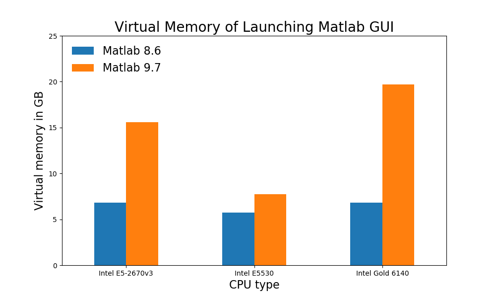
MATLAB memory needs upon opening the MATLAB GUI Desktop on different CPUs.¶
Please refer to the MATLAB documentation to learn how to use this software.
To submit submit a job for batch execution that will execute a MATLAB function that you have defined, you can create a submission script similar to:
#### submit_matlab.sh STOP ####
#!bin/bash
#$ -S /bin/bash
#$ -cwd
# error = Merged with joblog
#$ -o joblog.$JOB_ID
#$ -j y
# Edit the line below as needed
#$ -l h_data=10G,h_rt=1:00:00
# Add multiple cores/nodes as needed:
#$ -pe shared 1
# Email address to notify
#$ -M $USER@mail
# Notify when
#$ -m bea

# echo job info on joblog:
echo "Job $JOB_ID started on:  " `hostname -s`
echo "job $JOB_ID started on:  "  `date `


## commands here ##
. /u/local/Modules/default/init/modules.sh
module load matlab
module li
echo " "
export MCR_CACHE_ROOT=$TMPDIR
echo "MCR_CACHE_ROOT=$MCR_CACHE_ROOT"
echo " "

# substitute the command to run your code below:
echo "matlab -nojvm -nodisplay -nosplash -r MYMATLABFUNCTION >> output.$JOB_ID"
matlab -nojvm -nodisplay -nosplash -r MYMATLABFUNCTION >> output.$JOB_ID

# echo job info on joblog:
echo "Job $JOB_ID ended on:   " `hostname -s`
echo "Job $JOB_ID ended on:   " `date `
echo " "
#### submit_matlab.sh STOP ####
To submit MATLAB script from a terminal on the cluster, navigate to the directory where your MATLAB script is and use any one of the following scripts according to your needs:
$ /u/local/apps/submit_scripts/matlab_compile_and_submit_noSingleCompThreads.sh
$ /u/local/apps/submit_scripts/matlab_compile_and_submit.sh
$ /u/local/apps/submit_scripts/matlab_no_compile_submit_exclusive_change_dir.sh
$ /u/local/apps/submit_scripts/matlab_no_compile_submit_exclusive_dir.sh
$ /u/local/apps/submit_scripts/matlab_no_compile_submit_exclusive.sh
$ /u/local/apps/submit_scripts/matlab_no_compile_submit.sh
$ /u/local/apps/submit_scripts/matlab_no_compile_submit_v9.1.sh
to learn how to use them just issue, for example, for matlab_compile_and_submit_noSingleCompThreads.sh, issue:
$ /u/local/apps/submit_scripts/matlab_compile_and_submit_noSingleCompThreads.sh
which will give you:
Usage:
 /u/local/apps/submit_scripts/matlab_compile_and_submit_noSingleCompThreads.sh  [-t time in hours]
    [ -s number of processes ] [-m memory per process (in GB)]
    [-p parallel environment: 1 for shared 2 for distributed]
    [-a add file or entire directory to the deployable archive] ...
    [-a add other file or other entire directory to the deployable archive]
    [-I add directory to the list of included directories] ...
    [-I add other directory to the list of included directories]
    [-f main matlab function] [-f matlab function 2] ... [-f matlab function n]
    [-ns (to build a submission script without submitting the job)]
    [-nts (to not addtime stamp to cmd file name)]
    [-hp to run on owned nodes] [ --help ]
to submit the MATLAB script myscript.m or batch execution you can then use, for example:
$ /u/local/apps/submit_scripts/matlab_compile_and_submit_noSingleCompThreads.sh =t 3 -m 10 -f myscript.m
The following queue scripts are also available for MATLAB (however they are currently unsupported):
$ matlab.q
runs single or multi-processor in two steps: compile and execute. The matlab.q script will compile the MATLAB files into a stand-alone program so that the execution of MATLAB files on computers will not require a MATLAB license at run time. For serial or implicit multi-threaded MATLAB code, no extra work will be needed to run MATLAB .m files using matlab.q in most cases.
$ mcc.q
uses the MATLAB compiler to create a stand-alone executable. If you are using mcc.q interactively, it will ask you if you want the executable produced by mcc to use a single processor or not. If you are using mcc.q in command line mode, to create an executable that will run on a single processor specify this argument:
-R -singleCompThread
To run a previously generated matlab stand alone executable (generated with the MATLAB compiler) use:
$ matexe.q
runs a MATLAB stand-alone executable created with mcc.
Please refer to the MATLAB documentation to learn how to use this software.
Dispatch MATLAB batch jobs via the Parallel Computing Toolbox and the MATLAB Parallel Server running on the cluster. You can dispatch MATLAB batch jobs from a MATLAB desktop running either on your local computer or a Matlab desktop running on the cluster.
Please see MATLAB Access for University of California Los Angeles to lern how to install MATLAB on your local computer.
Note
Currently MATLAB version R2020b is supported on the Hoffman2 Cluster. Make sure to download locally this version of MATLAB.
Once you have installed MATLAB on your personal computer you will need to configure the local instance of the MATLAB Parallel Server so that it can dispatch jobs on the Hoffman2 Cluster. To do so follow these steps:
Transfer the archival file:
/u/local/apps/matlab/PARALLEL_TOOLBOX_SETUP/UCLA.nonshared.R2020b.zip
from the Hoffman2 Cluster to your local computer the file. Unzip the file in your local:
$MATLABROOT/toolbox/local
directory. This location will change with your specific OS. For example, on a Mac and for MATLAB version R2020b, open the Terminal application and at the command line issue:
$ cd /Applications/MATLAB_R2020b.app/toolbox/local
$ unzip ~/Downloads/UCLA.nonshared.R2020b.zip
Start MATLAB and at the MATLAB prompt issue:
>> rehash toolboxcache
>> configCluster
You will be prompted to enter your Hoffman2 Cluster username. Jobs will now be executed on Hoffman2.
If you decide to execute jobs locally use:
>> c = parcluster('local');
Log on the cluster so that you can open the MATLAB desktop (see: Interactive use). Get an interactive session with the needed resources (e.g., run-time, memory, number of cores), for example with:
$ qrsh -l h_rt=1:00:00,h_data=12G
start the MATLAB desktop with:
$ module load matlab/R2020b
$ matlab &
at the MATLAB prompt issue:
>> rehash toolboxcache
>> configCluster
Jobs will now be submitted via the scheduler, if you decide to execute them on the local node where your MATLAB desktop is running, type:
>> c = parcluster('local');
If you already have a MATLAB script that you would like to submit to the cluster from the terminal command line (i.e., without opening the MATLAB desktop) you can do so using the script:
$ /u/local/apps/submit_scripts/MATLAB_PARALLEL_BATCH_SUBMISSION/matlab_batch_parallel_job_submit.sh
to see how the script work issue:
$ /u/local/apps/submit_scripts/MATLAB_PARALLEL_BATCH_SUBMISSION/matlab_batch_parallel_job_submit.sh --help
to learn more see:
$ /u/local/apps/submit_scripts/MATLAB_PARALLEL_BATCH_SUBMISSION/README.HOWTO
Before running jobs on the cluster you should make sure to specify scheduler parameters to be passed to your job. To do so open MATLAB and type commads similar to what shown below (you will need to change the parameters to fit your job needs):
>> % Get a handle to the cluster
>> c = parcluster;

>> % Specify the walltime (e.g. 5 hours)
>> c.AdditionalProperties.WallTime = '05:00:00';

>> % Specify memory to use for MATLAB jobs
>> c.AdditionalProperties.MemUsage = '8G';

>> % Specify the number of GPU Nodes requested (currently limited to 1 node)
>> c.AdditionalProperties.GpuNodes = 1;

>> % Specify the type of GPU
>> c.AdditionalProperties.GpuType = 'V100';

>> % Specify special submissions flags (e.g., exclusive, highp, etc…)
>> c.AdditionalProperties.AdditionalSubmitArgs='-l exclusive -l highp'

>> % Save changes:
>> c.saveProfile

>> % Check current properties:
>> c.AdditionalProperties

>> % Change or remove one of the properties, e.g.:
>> c.AdditionalProperties.AdditionalSubmitArgs = '';
>> c.saveProfile
Submit simple matlab job that checks the location of your $HOME directory on the cluster:
>> % Get a handle to the cluster
>> c = parcluster;
>> % Submit job to query from which directory is MATLAB running on the cluster
>> j = c.batch(@pwd, 1, {}, 'CurrentFolder', '.', 'AutoAddClientPath',false);
>> % Query job for state
>> j.State
>> % If state is finished, fetch the results
>> j.fetchOutputs{:}
>> % Delete the job after results are no longer needed
>> j.delete
To retrieve a list of running or completed jobs and view results:
>> c = parcluster;
>> jobs = c.Jobs;
>> % Get a handle to the job with ID 2
>> j2 = c.Jobs(2);
>> % Fetch results for job with ID 2
>> j2.fetchOutputs{:}
Please refer to the MATLAB documentation to learn how to use this software.
Problems with the instructions on this section? Please send comments here.
NCO¶
“The NCO toolkit manipulates and analyzes data stored in netCDF-accessible formats, including DAP, HDF4, and HDF5. It exploits the geophysical expressivity of many CF (Climate & Forecast) metadata conventions, the flexible description of physical dimensions translated by UDUnits, the network transparency of OPeNDAP, the storage features (e.g., compression, chunking, groups) of HDF (the Hierarchical Data Format), and many powerful mathematical and statistical algorithms of GSL (the GNU Scientific Library). NCO is fast, powerful, and free.” – The NCO website
Start by requesting an interactive session with the needed resources (e.g., run-time, memory, number of cores, etc.), for example with:
qrsh -l h_data=2G,h_rt=1:00:00
To set up your environment to use NCO, use the module command:
module load nco
You will then be able to invoke NCO’s binaries (i.e., ncap2, ncatted, ncbo, ncclimo, nces, ncecat, ncflint, ncks, ncpdq, ncra, ncrcat, ncremap, ncrename, ncwa) from the command line.
Please refer to the NCO documentation to learn how to use this software.
To submit a job for batch execution which uses any of the NCO you will need to create a submission script similar to:
### NCO_submit.sh START ###
#!/bin/bash
#$ -cwd
# error = Merged with joblog
#$ -o joblog.$JOB_ID
#$ -j y
# Edit the line below to request the appropriate runtime and memory
# (or to add any other resource) as needed:
#$ -l h_rt=1:00:00,h_data=1G
# Add multiple cores/nodes as needed:
#$ -pe shared 1
# Email address to notify
#$ -M $USER@mail
# Notify when
#$ -m bea

# echo job info on joblog:
echo "Job $JOB_ID started on:   " `hostname -s`
echo "Job $JOB_ID started on:   " `date `
echo " "

# load the job environment:
. /u/local/Modules/default/init/modules.sh
module load NCO

# substitute the command to run the needed NCO command (e.g.: ncap2,
# ncatted, ncb,o ncclimo, nces, ncecat, ncflint, ncks, ncpdq, ncra,
# ncrcat, ncremap, ncrename or ncwa) below:
echo '$SAMPLECOMMAND'
$SAMPLECOMMAND

# echo job info on joblog:
echo "Job $JOB_ID ended on:   " `hostname -s`
echo "Job $JOB_ID ended on:   " `date `
echo " "
### NCO_submit.sh STOP ###
where you would replace the resources requested and the NCO command as needed. Save the NCO_submit.sh script in a location on your account from which you would like to submit your job, mark the script as an executable script with:
chmod u+x NCO_submit.sh
Submit the job with:
 qsub NCO_submit.sh

Please refer to the `NCO documentation <http://nco.sourceforge.net/nco.html>`__ to learn how to use this software.
Problems with the instructions on this section? Please send comments here.
Octave¶
GNU Octave is software featuring a high-level programming language, primarily intended for numerical computations. Octave helps in solving linear and nonlinear problems numerically, and for performing other numerical experiments using a language that is mostly compatible with MATLAB. For more information, see the GNU Octave website.
Start by requesting an interactive session with the needed resources (e.g., run-time, memory, number of cores, etc.), for example with:
$ qrsh -l h_data=2G,h_rt=1:00:00
To set up your environment to use Octave, use the module command:
$ module load octave
See How to use the module command for further information.
Please refer to the Octave documentation to learn how to use this software.
Problems with the instructions on this section? Please send comments here.
OpenSees¶
“OpenSees, the Open System for Earthquake Engineering Simulation, is an object-oriented, open source software framework. It allows users to create both serial and parallel finite element computer applications for simulating the response of structural and geotechnical systems subjected to earthquakes and other hazards. OpenSees is primarily written in C++ and uses several Fortran and C numerical libraries for linear equation solving, and material and element routines.” – OpenSees Wiki website.
On Hoffman2, OpenSees and OpenSeesMP is installed as an Apptainer container. This container is located on Hoffman2 at $H2_CONTAINER_LOC/h2-opensees_3.3.0.sif
You can use any text editor to make the appropriate input files for opensees.
Start by requesting an interactive session with the needed resources (e.g., run-time, memory, number of cores, etc.), for example with:
$ qrsh -l h_data=2G,h_rt=1:00:00
At the compute node shell prompt, enter:
$ module load apptainer
$ apptainer shell  $H2_CONTAINER_LOC/h2-opensees_3.3.0.sif
$ OpenSeesMP
Please see the OpenSees documentation to learn how to use this software.
To run OpenSees and OpenSeesMP, you will need to load Apptainer
The following queue script is available for opensees to run in Serial
### submit_opensees_ser.sh START ###
#!/bin/bash
#$ -cwd
# error = Merged with joblog
#$ -o joblog.$JOB_ID
#$ -j y
# Edit the line below to request the appropriate runtime and memory
# (or to add any other resource) as needed:
#$ -l h_rt=1:00:00
# Email address to notify
#$ -M $USER@mail
# Notify when
#$ -m bea

# echo job info on joblog:
echo "Job $JOB_ID started on:   " `hostname -s`
echo "Job $JOB_ID started on:   " `date `
echo "Job $JOB_ID will run on:  "
cat $PE_HOSTFILE
echo " "

# load the job environment:
. /u/local/Modules/default/init/modules.sh
module load apptainer

# Runing OpenSeesMP in serial
time apptainer exec  $H2_CONTAINER_LOC/h2-opensees_3.3.0.sif  OpenSeesMP sample.tcl  > output.$JOB_ID

# echo job info on joblog:
echo "Job $JOB_ID completed on:   " `hostname -s`
echo "Job $JOB_ID completed on:   " `date `
echo " "
### submit_opensees_ser.sh STOP ###
To use OpenSeesMP in parallel, you will need to load the intel module and use mpirun
### submit_opensees_par.sh START ###
#!/bin/bash
#$ -cwd
# error = Merged with joblog
#$ -o joblog.$JOB_ID
#$ -j y
# Edit the line below to request the appropriate runtime and memory
# (or to add any other resource) as needed:
#$ -l h_rt=1:00:00
# Email address to notify
#$ -M $USER@mail
# Notify when
#$ -m bea
#$ -pe dc* 8

# echo job info on joblog:
echo "Job $JOB_ID started on:   " `hostname -s`
echo "Job $JOB_ID started on:   " `date `
echo "Job $JOB_ID will run on:  "
cat $PE_HOSTFILE
echo " "

# load the job environment:
. /u/local/Modules/default/init/modules.sh
module load apptainer
module load intel

# Runing OpenSeesMP in parallel
`which mpirun` -np $NSLOTS apptainer exec  $H2_CONTAINER_LOC/h2-opensees_3.3.0.sif  OpenSeesMP sample.tcl  > output.$JOB_ID

# echo job info on joblog:
echo "Job $JOB_ID completed on:   " `hostname -s`
echo "Job $JOB_ID completed on:   " `date `
echo " "
### submit_opensess_par.sh STOP ###
Please see the OpenSees documentation to learn how to use this software.
Problems with the instructions on this section? Please send comments here.
Physics¶
CERN ROOT¶
ROOT is an object-oriented program and library developed by CERN. It was originally designed for particle physics data analysis and contains several features specific to this field, but it is also used in other applications such as astronomy and data mining. For more information, see the ROOT website.
Start by requesting an interactive session with the needed resources (e.g., run-time, memory, number of cores, etc.), for example with:
$ qrsh -l h_data=2G,h_rt=1:00:00
Use qrsh to obtain a session on a compute node. Then enter:
$ module load cern-root
$ root
To exit the cint C++ interpreter, at the ROOT prompt, enter:
.q
Problems with the instructions on this section? Please send comments here.
Geant4¶
“Geant4 is a toolkit for the simulation of the passage of particles through matter. Its areas of application include high energy, nuclear and accelerator physics, as well as studies in medical and space science. ” – Geant4
Start by requesting an interactive session with the needed resources (e.g., run-time, memory, number of cores, etc.), for example with:
$ qrsh -l h_data=5G,h_rt=1:00:00 -pe shared 1
To set up your environment to use Geant4, use the module command:
$ module load gcc/8.30
$ module load geant4
To test the installation:
$ module load gcc/8.30; module load geant4
$ cp -rp /u/local/apps/geant4/11.0.1/gcc-8.3.0/examples/basic/B1 ./
$ cd B1
$ mkdir build
$ cd build
$ cmake ..
Problems with the instructions on this section? Please send comments here.
Statistics¶
R¶
R is a programming language and free software environment for statistical computing and graphics supported by the R Foundation for Statistical Computing. The R language is widely used among statisticians and data miners for developing statistical software and data analysis. For more information, see the R-project website.
You can use any text editor to make the appropriate input files for R. RStudio, an IDE for R, can be used to prepare R scripts.
Request an interactive session with the needed resources (e.g., run-time, memory, number of cores, etc.), for example:
$ qrsh -l h_data=2G,h_rt=1:00:00
At the compute node shell prompt, enter:
$ module load R
$ R
To see which versions of R are installed on the cluster use:
$ module av R
to load a different version of R issue:
$ module load R/VERSION
where: VERSION is the needed version.
Please refer to the R documentation to learn how to use this software.
Problems with the instructions on this section? Please send comments here.
Jupyter Notebook/Lab can be used to develop and run R very effectively. After opening a Jupyter Notebook/Lab on your locally running browser while harnessing the computing power of the Hoffman2 Cluster (see: Connecting via Jupyter Notebook/Lab to learn how to do so), you can start an R notebook by selecting the needed version of R from the New pulldown menu.
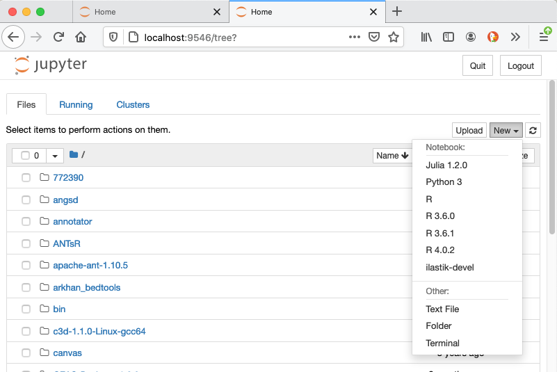
How to start an R Jupyter Notebook by clicking on the New pulldown menu in the classic Jupyter Notebook view.¶
Within a Jupyter Lab, an R notebook can be started clicking on the Launcher R icon.
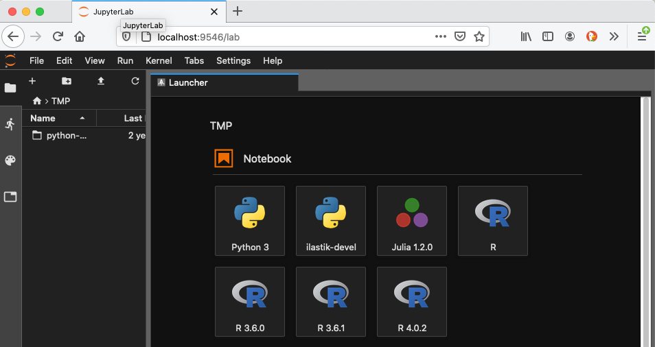
How to start an R Jupyter Notebook by clicking on the R icon on in the Jupyter Lab Launcher window.¶
Jupyter notebooks combine the many aspects of classic IDEs and they have the added bonus of displaying results very fast as the graphic is rendered on the local client.
R Jupyter Notebook with R code implementing the booostrapping approximation of \({\pi}\) and a plot showing a visual approximation of \({\pi}\)¶
Please refer to the R documentation to learn how to use this software.
Problems with the instructions on this section? Please send comments here.
There are several ways to submit R batch jobs on the cluster:
using the wrapper script, R_job_submitter.sh, that allows you to request a specific version of R and computational resources
using the sample submission script, R_submit.sh, provided below
using R.q which will force you to use a fixed version of R
if you intend to run a batch job using the version of R provided with Rstudio Server please refer to RStudio Server
$ /u/local/apps/submit_scripts/R_job_submitter.sh
the script allow you to select the R version and pass several arguments as shown below:
Usage:
 /u/local/apps/submit_scripts/R_job_submitter.sh [-n R script name]
   [-m memory per slot (in GB)] [-t time in hours] [-hp to run on owned nodes]
   [-ex to run exclusively] [-s number of slots] [-v R version]
   [-arg argument 1 to pass to R script] [-arg argument 2 to pass to R script]
   ... [-arg argument n to pass to R script]
   [-ns (to build a submission script without submitting the job)]
   [-nts (to not add time stamp to cmd file name)] [ --help ]
For example, to submit an R script, myscript.R, using R version 4.0.2, 4GB of memory and a runtime of 1 hour:
$ /u/local/apps/submit_scripts/R_job_submitter.sh -v 4.0.2 -m 4 -t 1 -n myscript.R
the command above will return something similar to:
Running myscript.R on 1 processes each with 4GB of memory for 1 hours
Your job 4264527 ("myscript_2020-09-02_18-11-23.cmd") has been submitted
this means that a submission script named myscript_2020-09-02_18-11-23.cmd was generated and submitted to the queues. To remove the time stamp from the submission script name you can add the -nts flag to your command, i.e.:
$ /u/local/apps/submit_scripts/R_job_submitter.sh -v 4.0.2 -m 4 -t 1 -n myscript.R -nts
you can check the status of your submission with:
$ myjobs
To submit a job for batch execution with R, you will need to create a submission script similar to:
### R_submit.sh START ###
#!/bin/bash
#$ -cwd
#$ -o  joblog.$JOB_ID
#$ -j y
#  Resources requested
#  PLEASE CHANGE THE RESOURCES REQUESTED AS NEEDED:
#$ -l h_data=4G,h_rt=1:00:00
#  PLEASE CHANGE THE NUMBER OF CORES REQUESTED AS NEEDED:
#$ -pe shared 1
#  Email address to notify
#$ -M $USER@mail
#$ -m bea
# #$ -V

#
# Output job info on joblog file:
#
echo " "
echo "Job myscript, ID no. $JOB_ID started on:   "` hostname -s `
echo "Job myscript, ID no. $JOB_ID started at:   "` date `
echo " "

#
# Set up job environment:
#
. /u/local/Modules/default/init/modules.sh
module load R
# SHOULD YOU NEED TO LINK TO ANY PARTICULAR LIBRARY, USE:
# export LD_LIBRARY_PATH=/path/to/libdir/if/needed:$LD_LIBRARY_PATH
# SHOULD YOU NEED TO CHANGE THE LOCATION OF THE R TEMPORARY DIRECTORY:
# if [ ! -d $SCRATCH/R_scratch ]; then
#    mkdir $SCRATCH/R_scratch
# fi
# export TMPDIR=$SCRATCH

#
# Run the R script:
#
echo " "
#  (SUBSTITUTE THE NAME OF YOUR R SCRIPT AND OUTPUT BELOW):
echo R CMD BATCH --no-save --no-restore  myscript.R output.$JOB_ID
#  (SUBSTITUTE THE NAME OF YOUR R SCRIPT AND OUTPUT BELOW):
/usr/bin/time -v R CMD BATCH --no-save --no-restore  myscript.R  output.$JOB_ID
#
echo " "
echo "Job myscript, ID no. $JOB_ID finished at:  "` date `
echo " "
### R_submt.sh STOP ###
where, in the highlighted lines, you would replace the resources requested and the name of the R script and output file as needed. Save the R_submit.sh script in a location on your account from which you would like to submit your job, mark the script as an executable script with:
$ chmod u+x R_submit.sh
Submit the job with:
$ qsub R_submit.sh
The script R.q is also available to submit R serial jobs.
Please refer to the R documentation to learn how to use this software.
Problems with the instructions on this section? Please send comments here.
R Libraries¶
R includes a set of base packages and additional add-on libraries. Several additional libraries have already been installed in any version of R available on the Hoffman2 Cluster (to see all versions currently available use: modules_lookup -m R). To see a list of the installed libraries, at the R command prompt, enter:
> library()
Additional libraries can be installed in each user directory where they are available to the particular user who has performed the installation. If a group project space is available, R libraries of common use for a group can also be installed in a group project space where they can be made available to all the users of such group.
Additional libraries not already installed with the versions of R available on the cluster (to see all versions currently available use: modules_lookup -m R), can be installed in a personal R library directory. To install a library and its dependencies in this location you will need to run R interactively and issue at the R command line:
> install.packages('package_name', dependencies=TRUE)
R will inform you that you can’t write to the global directory, and ask if you want to use a personal library instead. When prompted answer yes. R will then prompt you with a path and ask if you want to use this. When prompted answer yes. R will then install the library in this location.
See the R Installation and Administration guide for more information on how to customize the install.packages command (for example you could add the repository by including in the argument of your install.packages command the string: repos=”http://cran.r-project.org”).
To see a list of directories that R searches for libraries issue at the R prompt:
> .libPaths()
Problems with the instructions on this section? Please send comments here.
If your group has purchased additional storage and you would like to perform an installation of certain R libraries that would be available to all of your group, you should follow these steps:
Request the creation of a shared directory in your group space by opening a ticket at: https://support.idre.ucla.edu/helpdesk or sending an email to hpc@ucla.edu.
Create an
R/<VERSION>(to see all versions currently available use:modules_lookup -m R) directory in your project directory, for example if your project group is calledbruinsponsor, the shared directory is calledappsand the version ofRfor which you intend to install supplemental libraries is4.2.2, compiled withgcc/10.2.0(available via the modulefiles:module load gcc/10.2.0; module load R/4.2.2), you would issue:Note
In the current example the project common directory is:
/u/project/bruinsponsor/apps/R/4.2.2_gcc_10.2.0You will need to update the name of this directory to reflect the name of your project directory and the desired version of R. To see all version of R available use the command:
$ modules_lookup -m Rin the code below update the name of the common directory as needed.
$ mkdir -p /u/project/bruinsponsor/apps/R/4.2.2_gcc_10.2.0 # change the name as needed
Install packages the project common directory:
Note
In the current example the project common directory is:
/u/project/bruinsponsor/apps/R/4.2.2_gcc_10.2.0in the code below update the name of the common directory as needed.
$ qrsh -l h_data=10G
$ module load gcc/10.2.0; module load R/4.2.2
$ mkdir -p /u/project/bruinsponsor/apps/R/4.2.2_gcc_10.2.0
$ export R_LIBS_SITE=/u/project/bruinsponsor/apps/R/4.2.2_gcc_10.2.0:$R_LIBS_SITE
$ # start R:
$ R   # at the R prompt check R libraries location:
> .libPaths()  # this should give you:
[1] "/u/home/j/joebruin/R/x86_64-pc-linux-gnu-library-RH7/4.2.2/intel2022.1.1_gcc10.2.0"
[2] "/u/project/bruinsponsor/apps/R/4.2.2_gcc_10.2.0"
[3] "/u/local/apps/R/4.2.2/gcc10.2.0_intel2022.1.1/lib64/R/library"
> # start the library installation, e.g., for package smile:
> install.packages('smile',lib=.libPaths()[2])
> # or for packages from Bioconductor:
> if (!requireNamespace("BiocManager", quietly = TRUE))
+ install.packages("BiocManager",lib = .libPaths()[2])
> BiocManager::install(c("BiocParallel", "callr", "xfun","xml2"), update = TRUE, lib = .libPaths()[2])
Warning
In general only one user in the group will have write permission to the
/u/project/bruinsponsor/appsdirectory.Use packages from this common directory:
Note
In the current example the project common directory is:
/u/project/bruinsponsor/apps/R/4.2.2_gcc_10.2.0in the code below please update the name of the common directory to reflect your own.
$ qrsh -l h_data=10G
$ module load gcc/10.2.0; module load R/4.2.2
$ export R_LIBS_SITE=/u/project/bruinsponsor/apps/R/4.2.2_gcc_10.2.0:$R_LIBS_SITE
$ R   # start R and at the R prompt check R libraries location:
> .libPaths()  # this should give you:
[1] "/u/home/j/joebruin/R/x86_64-pc-linux-gnu-library-RH7/4.2.2/intel2022.1.1_gcc10.2.0"
[2] "/u/project/bruinsponsor/apps/R/4.2.2_gcc_10.2.0"
[3] "/u/local/apps/R/4.2.2/gcc10.2.0_intel2022.1.1/lib64/R/library"
Problems with the instructions on this section? Please send comments here.
Note
The R library rJava, a low-level R to Java interface, depends on the exact java version on the computing node. As it may happen that the default version of java on different computational nodes slightly differs (which may be due to an update in progress), rJava may appears to not work on some nodes. In this cases we suggest to modify the R command as follows:
$ qrsh -l h_data=5G   # request enough memory to start java
$ module load R
$ R CMD javareconf -e
$ R CMD BATCH filename
For sh-based scripts use:
$ . /u/local/Modules/default/init/modules.sh
$ module load R
$ R CMD javareconf -e
$ R CMD BATCH filename
For csh-based scripts use:
$ source /u/local/Modules/default/init/modules.csh
$ module load R
$ R CMD javareconf -e
$ R CMD BATCH filename
Note
You may need to update the module load R command to reflect a preferred version of R. To see all version of R available use the command:
$ modules_lookup -m R
Please refer to the R documentation to learn how to use this software.
Problems with the instructions on this section? Please send comments here.
Additional libraries, that are of relevant usage to the Hoffman2 community, can also be installed in the central repository upon request. See the Software installation page.
Problems with the instructions on this section? Please send comments here.
RStudio¶
RStudio is an integrated development environment for R, a programming language for statistical computing and graphics. For more information, see the RStudio website.
On the Hoffman2 Cluster, you can run either the RStudio IDE or RStudio Server versions.
RStudio IDE¶
RStudio IDE (formerly known as RStudio Desktop) is a standalone desktop version that can be launched on a compute node on the Hoffman2 cluster. To open the RStudio IDE GUI, users need to follow the steps outlined in the opening GUI applications section. RStudio Desktop supports all versions of R that are installed on the Hoffman2 cluster.
Warning
To open the RStudio IDE GUI, you MUST connected to the Hoffman2 Cluster either via a remote desktop or via terminal and SSH having followed directions on how to open GUI applications. If you do not follow these steps, you will not be able to open the RStudio GUI.
To run Rstudio, first start an interactive session using qrsh requesting the correct amount of resources (memory and/or cores, computing time, etc.) that your R scripts will be needing.
Request an interactive session with the needed resources (e.g., run-time, memory, number of cores, etc.), for example, to request one computational core with 2GB or memory for 1 hour, issue at cluster command prompt:
$ qrsh -l h_data=5G,h_rt=1:00:00
At the compute node shell prompt, enter:
$ module load Rstudio
$ rstudio &
Note
The RStudio module will load into your environment the current default version of R on the cluster unless you have an R module already loaded. To witch versions of R simply load the needed R module before opening Rstudio.
Problems with the instructions on this section? Please send comments here.
RStudio Server¶
RStudio Server allows users to start an RStudio session on a compute node that can be accessed through a web browser running on the local computer. As RStudio Server is executed inside a software container accessible via Apptainer, the version of R available to this version of RStudio is limited to the one installed within the container. RStudio Server bypasses the need to access a GUI application remotely, thus avoiding any associated inefficiencies.
The RStudio Server application is ran using Apptainer on a compute node to be rendered on a web browsed running on your local machine.
To find available RStudio container versions on the Hoffman2 Cluster issue the following commands from a terminal:
module load apptainer
ls $H2_CONTAINER_LOC/h2-rstudio*sif
You can follow these steps to start a RStudio Server session:
Open a terminal and connect to the Hoffman2 Cluster, at the cluster command prompt issue:
# get an interactive job
qrsh -l h_data=10G
# Create small tmp directories for RStudio to write into
mkdir -pv $SCRATCH/rstudiotmp/var/lib
mkdir -pv $SCRATCH/rstudiotmp/var/run
mkdir -pv $SCRATCH/rstudiotmp/tmp
#Setup apptainer
module load apptainer
## Run rstudio
##
## NOTE: you can change the version of R by selecting a different RStudio container
##
##       use:
##
##            module load apptainer; ls $H2_CONTAINER_LOC/h2-rstudio*sif
##
##       to see which versions are available
##
apptainer run -B $SCRATCH/rstudiotmp/var/lib:/var/lib/rstudio-server -B $SCRATCH/rstudiotmp/var/run:/var/run/rstudio-server -B $SCRATCH/rstudiotmp/tmp:/tmp $H2_CONTAINER_LOC/h2-rstudio_4.1.0.sif
## This command will display the following information:
##
## This is the Rstudio server container running R 4.3.2 from Rocker
##
## This is a separate R version from the rest of Hoffman2
## When you install libraries from this Rstudio/R, they will be in ~/R/APPTAINER/h2-rstudio_4.3.2
##
##
## Your Rstudio server is running on:  <NODE>
## It is running on PORT:  <PORT>
##
## Open a SSH tunnel on your local computer by running:
##  ssh -N -L <PORT>:<NODE>:<PORT> <YOUR_H2C_USERNAME>@hoffman2.idre.ucla.edu
##
## Then open your web browser to  http://localhost:<PORT>
##
## Your Rstudio Password is:  <TEMPORARY_PASSWORD>
## Please run [CTRL-C] on this process to exit Rstudio
##
## You will need to run the `ssh -N -L ...` command on a separate terminal on your local computer
##
##    ***USE THE <TEMPORARY_PASSWORD> WHEN RSTUDIO SERVER OPENS ON YOUR LOCAL BROWSER***
##
After the
apptainer run ...command you will be prompted with information regarding the version of R and Rstudio, the node where the Rstudio session is running and the port through which the application is listening. There will also be three lines of instructing you on how to initiate an SSH tunnel on your local computer in order to be able to connect with your local browser to the Rstudio session running remotely on the cluster compute node, you will also be prompted with the temporary password which you will need to open the RStudio Server session on your browser. These instructions are relevant for the next steps and are highlighted in the sample output of theapptainer run ...command given below:$ apptainer run -B $SCRATCH/rstudiotmp/var/lib:/var/lib/rstudio-server -B $SCRATCH/rstudiotmp/var/run:/var/run/rstudio-server -B $SCRATCH/rstudiotmp/tmp:/tmp $H2_CONTAINER_LOC/h2-rstudio_4.1.0.sif INFO: Converting SIF file to temporary sandbox... This is the Rstudio server container running R 4.3.2 from Rocker This is a separate R version from the rest of Hoffman2 When you install libraries from this Rstudio/R, they will be in ~/R/APPTAINER/h2-rstudio_4.3.2 Your Rstudio server is running on: <NODE> It is running on PORT: <PORT> Open a SSH tunnel on your local computer by running: ssh -N -L <PORT>:<NODE>:<PORT> <YOUR_H2C_USERNAME>@hoffman2.idre.ucla.edu Then open your web browser to http://localhost:<PORT> Your Rstudio Password is: <TEMPORARY_PASSWORD> Please run [CTRL-C] on this process to exit Rstudio
where
<NODE>is the name of the actual compute node where the Rstudio session is running, <PORT> is the number corresponding to the port on which the RStudio Server is running,<YOUR_H2C_USERNAME>is your Hoffman2 Cluster User ID and<TEMPORARY_PASSWORD>is the temporary password you will need to log onto the RStudion Server session. Make note of these instructions as they will be needed in the next step of the setup.Important
The version of R that you are running on RStudio Server does not correspond to any of the R versions available on the cluster via:
module av R. If you would like to run batch jobs with this version of R you will need to follow the information given in the tab of RStudio Server.Open a new terminal window on your local computer and initiate the SSH tunnel as indicated in the terminal in which the
apptainer run ...command was executed. For example, userjoebruinwhose RStudion Server which started on node n1234 and on port 8787, will need to run the SSH Port Forwarding command:
$ ssh -N -L 8787:n1234:8787 joebruin@hoffman2.idre.ucla.eduAfter issuing the SSH Port Forwarding command you will be prompted for your password and, if the SSH tunnel is successful the prompt will not return on this terminal (until the RStudio Server session is running). If you desire to free your terminal for other uses you can issue instead:
$ ssh -f -N -L <PORT>:<NODE>:<PORT> <YOUR_H2C_USERNAME>@hoffman2.idre.ucla.eduwhere
<NODE>is the name of the actual compute node where the Rstudio session is running,<PORT>is the number corresponding to the port on which the RStudio Server is running,<YOUR_H2C_USERNAME>is your Hoffman2 Cluster User ID.
You can also run the version of R available with RStudio Server in a submitted batch job. Your submission script will need to start R from the software container where RStudio Server is installed. The following code is an example of a SGE job script that will submit a R batch job using the version of R inside of the RStudio container. You can use all the R libraries and packages that you have already installed from within an RStudio Server session.
You may need to modify the instructions given in below to match the particular R container you would want to use. To find available RStudio container versions on the Hoffman2 Cluster issue the following commands from a terminal:
module load apptainer
ls $H2_CONTAINER_LOC/h2-rstudio*sif
### submit_rstudio.sh START ###
#!/bin/bash
#$ -cwd
#$ -o  joblog.$JOB_ID
#$ -j y
#  Resources requested
#  PLEASE CHANGE THE RESOURCES REQUESTED AS NEEDED:
#$ -l h_data=10G,h_rt=1:00:00
#  PLEASE CHANGE THE NUMBER OF CORES REQUESTED AS NEEDED:
#$ -pe shared 1
#  Email address to notify
#$ -M $USER@mail
#$ -m bea

#
# Output job info on joblog file:
#
echo " "
echo "Job myscript, ID no. $JOB_ID started on:   "` hostname -s `
echo "Job myscript, ID no. $JOB_ID started at:   "` date `
echo " "

#
# Set up job environment:
#
. /u/local/Modules/default/init/modules.sh
module load apptainer

# Export R Libs directory
## NOTE YOU MAY NEED TO UPDATE THE DEFINITION OF R_LIBS_USER TO
## MATCH THE VERSION OF R YOU ARE USING (IF NOT USING h2-rstudio_4.1.0.sif)
export R_LIBS_USER=$HOME/R/APPTAINER/h2-rstudio_4.1.0

#
# Run the job:
#
## REMEMBER TO SUBSTITUTE THE NAME OF THE R SCRIPT YOU INTEND TO RUN IN THE TWO LINES BELOW &
## TO CHANGE THE RSTUDIO SERVER CONTAINER IF A DIFFERENT VERSION OF R IS NEEDED (TO SEE AVAILABLE
## VERSIONS OF R ISSUE: module load apptainer; ls $H2_CONTAINER_LOC/h2-rstudio*sif)
echo "/usr/bin/time -v apptainer exec $H2_CONTAINER_LOC/h2-rstudio_4.1.0.sif R CMD BATCH --no-save --no-restore myRtest.R output.$JOB_ID"
/usr/bin/time -v apptainer  exec $H2_CONTAINER_LOC/h2-rstudio_4.1.0.sif R CMD BATCH --no-save --no-restore myRtest.R output.$JOB_ID

echo " "
echo "Job myscript, ID no. $JOB_ID finished at:  "` date `
echo " "
### submit_rstudio.sh STOP ###
If you installed many R packages from within RStudio Server, you will want to run any R batch job with the same version of R and R packages.
Problems with the instructions on this section? Please send comments here.
Stata¶
Stata is a general-purpose statistical software package. Most of its users work in research, especially in the fields of economics, sociology, political science, biomedicine, and epidemiology. For more informatio, see the Stata website.
Note
To open the graphical user interface (GUI) of Stata, xstata, you will need to have connected to the Hoffman2 Cluster either via a remote desktop or via terminal and SSH having followed directions on how to open GUI applications. Alternatively you can open the text-based Stata interface.
Request an interactive session with the needed resources (e.g., run-time, memory, number of cores, etc.), for example:
$ qrsh -l h_data=2G,h_rt=1:00:00
After getting into the insteractive session, if you will be testing the parallel version, you will want to load the scheduler environmental variables (such as $NSLOTS for the number of parallel workers, etc._:
$ . /u/local/bin/set_qrsh_env.sh
To run Xstata interactively with its GUI interface, enter:
$ module load stata
$ xstata-se &
Or, for the multi-processor version of Xstata, enter:
$ module load stata
$ xstata-mp &
To run Stata interactively without its GUI interface, enter:
$ module load stata
$ stata-se
Or, for the multi-processor version of Stata:
$ module load stata
$ stata-mp
Stata writes temporary files to the directory /tmp or, if the $TMPDIR environmental variable is set, to the location pointed to by such variable. During a batch job, the $TMPDIR is set by the scheduler and points to a temporary directory located on the hard disk on the node where the job is running.
Should you need to have stata write its temporary files somewhere else then the locations indicated above, you can do by defining the $STATATMP before starting your stata session. On bash/sh shells you can do so by issuing:
$ export STATATMP=/path/to/your/stata/tmpdir
$ setenv STATATMP /path/to/your/stata/tmpdir
where: /path/to/your/stata/tmpdir should be substituted with an actual path on the cluster. If you intend to use your scratch directory, /path/to/your/stata/tmpdir should be set to $SCRATCH.
To verify the current location of the temporary directory Stata is using, you can issue at the Stata command prompt the following commands:
. tempfile junk
or:
. display "`junk'"
System environmental variables such as the location of your scratch on the cluster ($SCRATCH), or within a batch job contest, the job ID number, $JOB_ID, or for array jobs the task ID number, $SGE_TASK_ID, can be accessed from stata via macros. For example, to use $SCRACT within an interactive stata session or a stata do file:
. local scratch : env SCRATCH
. display "`scratch'"
and to change to $SCRACTH within an interactive stata session or a stata do file:
. cd `scratch'
To access either $JOB_ID or $SGE_TASK_ID from within an interactive stata session or a stata do file:
. local jid : env JOB_ID
. display `jid'
or:
. local tid : env SGE_TASK_ID
. display `tid'
To install in your $HOME directory and manage user-written additions from the net, use the stata command net. To learn more at the stata command prompt, issue:
. help net
The contributed commands from the Boston College Statistical Software Components (SSC) archive are installed in the users $HOME directory as needed. To do so, start an interactive session of Stata and at its command prompt issue:
. ssc install pagkage-name
To check the location on your $HOME directory of stata packages, at the stata command prompt issue:
. sysdir
To check the locally installed packages, issue at the stata command prompt:
. ado
Please refer to the Stata documentation to learn how to use Stata.
To run Stata in batch you need to create an input script with a .do extension, the script will contain the Stata commands you would use at the Stata interactive prompt.
To submit a Stata script, say myscript.do, for batch executation you can create a script similar to:
#### stata_submit.sh START ####
#!/bin/bash
#$ -cwd
#$ -o joblog.$JOB_ID
#$ -j y
# Resources requested:
# UPDATE THE VALUE BELOW TO REFLECT YOUR NEEDS
#$ -l h_data=1g,h_rt=300
# UPDATE THE VALUE BELOW TO REFLECT YOUR NEEDS
#$ -pe shared 4
# Email address to notify
#$ -M $USER@mail
#$ -m bea

echo ""
echo "Job $JOB_ID started on: "` hostname -s `
echo "Job $JOB_ID started at: "` date `
echo ""
#
. /u/local/Modules/default/init/modules.sh
module load stata

# Tell stata how many processors to use ::

if [ -e ./profile.do ]; then
echo "set processors $NSLOTS" > profile.do
fi
cat ./profile.do
echo ""


#
# Run the user program
# CHANGE THE NAME OF THE STATA SCRIPT BELOW:

stata-mp -b do myscript.do 2>&1 > myscript.out.$JOB_ID


echo ""
echo "Job $JOB_ID ended on: "` hostname -s `
echo "Job $JOB_ID ended at: "` date `
echo ""
#### stata_submit.sh END ####
where you would replace the resources requested and Stata script name, myscript.do and the resources requested as needed. Save the stata_submit.sh script in a location on your account from which you would like to submit your job, mark the script as an executable script with:
$ chmod u+x stata_submit.sh
Submit the job with:
$ qsub stata_submit.sh
If you have to run a stata task multiple times using the same do file but changing, for example, a parameter within the study you can take advantage of the scheduler built-in job array capability which lets you submits such series of tasks with a single job submission.
A sample submission script (stata_jobarray_submission.sh) for such array job is shown here (where in bold are elements that you may likely want to adapt to your own situation):
#### stata_jobarray_submit.sh START ####
#!/bin/bash
#$ -cwd
#$ -o joblog.$JOB_ID.$TASK_ID
#$ -j y
# Resources requested:
# UPDATE THE VALUE BELOW TO REFLECT YOUR NEEDS
#$ -l h_data=1g,h_rt=300
# UPDATE THE VALUE BELOW TO REFLECT YOUR NEEDS
#$ -pe shared 4
# Email address to notify
#$ -M $USER@mail
#$ -m bea
# UPDATE THE VALUES BELOW TO REFLECT YOUR NEEDS
#$ -t 1-7:1

echo ""
echo "Job $JOB_ID started on: "` hostname -s `
echo "Job $JOB_ID started at: "` date `
echo ""
#
. /u/local/Modules/default/init/modules.sh
module load stata

# Tell stata how many processors to use ::

if [ -e ./profile.do ]; then
echo "set processors $NSLOTS" > profile.do
fi
cat ./profile.do
echo ""

echo "Task id is $SGE_TASK_ID"
echo ""

#
# Run the user program
# CHANGE THE NAME OF THE STATA SCRIPT BELOW:
cp -p ./batch_test.do ./batch_test_$SGE_TASK_ID.do
stata-mp -b do myscript.do $SGE_TASK_ID 2>&1 > myscript.out.${JOB_ID}.${SGE_TASK_ID}


echo ""
echo "Job $JOB_ID.$TASK_ID ended on: "` hostname -s `
echo "Job $JOB_ID.$TASK_ID ended at: "` date `
echo ""
#### stata_jobarray_submit.sh END ####
where you would replace the resources requested and Stata script name, myscript.do and the resources requested as needed. Save the stata_submit.sh script in a location on your account from which you would like to submit your job, mark the script as an executable script with:
$ chmod u+x stata_jobarray_submit.sh
Submit the job with:
$ qsub stata_jobarray_submit.sh
Should the run-time of your tasks be very short, you should group set of tasks as described in: :ref: How do I pack multiple job-array tasks into one run?
Finally, the following queue script is available for submitting Stata bath jobs:
stata.q
runs stata-mp on 1-8 processors.
Please refer to the Stata documentation to learn how to use Stata.
Problems with the instructions on this section? Please send comments here.
Visualization and rendering¶
GnuPlot¶
GnuPlot is a command-line program that can generate two- and three-dimensional plots of functions, data, and data fits. The program runs on all major computers and operating systems. For more information, see the GnuPlot website.
To run GnuPlot interactively you must connect to the cluster login node with X11 forwarding enabled. Then use qrsh to obtain an interactive compute node.
Note
To run GnuPlot you will need to have connected to the Hoffman2 Cluster either via a Remote desktop or via terminal and SSH having followed directions to Opening GUI applications.
Start by requesting an interactive session with the needed resources (e.g., run-time, memory, number of cores, etc.), for example with:
qrsh -l h_data=2G,h_rt=1:00:00
Then enter:
gnuplot
Please see the Gnuplot documentation to learn how to use this software.
Problems with the instructions on this section? Please send comments here.
GRACE¶
“Grace is a WYSIWYG tool to make two-dimensional plots of numerical data. It runs under various (if not all) flavors of Unix with X11 and M*tif (LessTif or Motif). It also runs under VMS, OS/2, and Windows (95/98/NT/2000/XP). Its capabilities are roughly similar to GUI-based programs like Sigmaplot or Microcal Origin plus script-based tools like Gnuplot or Genplot. Its strength lies in the fact that it combines the convenience of a graphical user interface with the power of a scripting language which enables it to do sophisticated calculations or perform automated tasks.” - GRACE Documentation website
You can use any text editor to make the appropriate input files for GRACE.
To run GRACE interactively you must connect to the cluster login node with X11 forwarding enabled. Then use qrsh to obtain an interactive session.
Note
To run GRACE you will need to have connected to the Hoffman2 Cluster either via a Remote desktop or via terminal and SSH having followed directions to Opening GUI applications.
Start by requesting an interactive session with the needed resources (e.g., run-time, memory, number of cores, etc.), for example with:
qrsh -l h_data=2G,h_rt=1:00:00
Then enter:
xmgrace
Problems with the instructions on this section? Please send comments here.
Graphviz¶
“Graphviz is open source graph visualization software. Graph visualization is a way of representing structural information as diagrams of abstract graphs and networks. It has important applications in networking, bioinformatics, software engineering, database and web design, machine learning, and in visual interfaces for other technical domains.” -Graphviz website
Note
To run Graphviz you will need to have connected to the Hoffman2 Cluster either via a Remote desktop or via terminal and SSH having followed directions to Opening GUI applications.
Start by requesting an interactive session with the needed resources (e.g., run-time, memory, number of cores, etc.), for example with:
qrsh -l h_data=2G,h_rt=1:00:00
To set up your environment to use Graphviz, use the module command:
module load graphviz
See Environmental modules for further information.
Problems with the instructions on this section? Please send comments here.
IDL¶
IDL, short for Interactive Data Language, is a programming language used for data analysis. It is popular in particular areas of science, such as astronomy, atmospheric physics and medical imaging. See the IDL webpage for more information.
You can use any text editor to make the appropriate input files for IDL.
To run IDL interactively you must first connect to the cluster login node with X11 forwarding enabled. Then use qrsh to obtain an interactive session.
Note
To run IDL you will need to have connected to the Hoffman2 Cluster either via a Remote desktop or via terminal and SSH having followed directions to Opening GUI applications.
Start by requesting an interactive session with the needed resources (e.g., run-time, memory, number of cores, etc.), for example with:
qrsh -l h_data=2G,h_rt=1:00:00
When the interactive session is granted enter at the command prompt of the compute node:
module load idl
idl
Please notice: IDL scripts (containing IDL commands and ending with a .pro extension) can be executed at the IDL command line.
Problems with the instructions on this section? Please send comments here.
ImageMagick¶
ImageMagick is a free and open-source software suite for displaying, creating, converting, modifying, and editing raster images. It can read and write over 200 image file formats. For more information, see ImageMagick website.
You can use any text editor to make the appropriate input files for ImageMagick.
To run ImageMagick interactively you must connect to the cluster login node with X11 forwarding enabled. Then use qrsh to obtain an interactive compute node.
Note
To run ImageMagick you will need to have connected to the Hoffman2 Cluster either via a Remote desktop or via terminal and SSH having followed directions to Opening GUI applications.
Start by requesting an interactive session with the needed resources (e.g., run-time, memory, number of cores, etc.), for example with:
qrsh -l h_data=2G,h_rt=1:00:00
Then enter:
image-magick-command {see options}
where image-magick-command is one of the ImageMagick programs.
Each ImageMagick program is invoked by a separate command. To run an ImageMagick program, either enter the command that invokes it at the command line shell prompt, or use it in a script file and execute your script.
Documentation exist for all the ImageMagick commands.
For a list of commands, issue:
man ImageMagick
For image settings and image operators, issue:
man display
Each ImageMagick program is invoked by a separate command. To run an ImageMagick program, either enter the command that invokes it or use it in a script file. Not all ImageMagick commands are available in batch (e.g., display and import do not run in batch).
The easiest way to run ImageMagick in batch from the login node is to use the queue scripts. See Submitting batch jobs for a discussion of the queue scripts and how they are used.
Use the job.q script to create a job scheduler command file for your script that contains an ImageMagick command and options.
See Submitting batch jobs for guidelines to follow to create the required UGE command file. Alternatively, you could create an UGE command file with the queue script listed above. After saving the command file, you can modify it if necessary. See Additional tools for a list of the most commonly used UGE commands.
Problems with the instructions on this section? Please send comments here.
Maya¶
“3D computer animation, modeling, simulation, and rendering software ” – Autodesk Maya
Note
To run Autodesk’s Maya you will need to have connected to the Hoffman2 Cluster either via a Remote desktop or via terminal and SSH having followed directions to Opening GUI applications.
After requesting an interactive session (remember to specify a runtime, memory, number of cores, etc. as needed), for example with:
qrsh -l h_rt=1:00:00,exclusive
You can check the available versions of Autodesk’s Maya with:
module av maya
Load the default version of Maya in your environment with:
module load maya
To load a different version, issue:
module load maya/VERSION
where VERSION is replaced by the desired version of Maya.
To invoke Maya:
maya &
Please refer to Autodesk’ Maya documentation to learn how to use this software Autodesk’ Maya documentation.
To submit a job for batch execution which uses any of the Autodesk’ Maya you can use the script:
/u/local/apps/submit_scripts/Render_job_submitter.sh
to learn how to use the script you can issue:
/u/local/apps/submit_scripts/Render_job_submitter.sh --help
Problems with the instructions on this section? Please send comments here.
NCAR¶
“The NCAR Command Language (NCL), a product of the Computational & Information Systems Laboratory at the National Center for Atmospheric Research (NCAR) and sponsored by the National Science Foundation, is a free interpreted language designed specifically for scientific data processing and visualization.” -NCL website
Note
To run NCL having followed directions to Opening GUI applications.
After requesting an interactive session with the needed resources (e.g., run-time, memory, number of cores, etc.), for example with:
qrsh -l h_data=2G,h_rt=1:00:00
Then enter:
/u/local/apps/ncl/current/bin/ncl
Problems with the instructions on this section? Please send comments here.
OpenDX¶
OpenDX is a programming environment for data visualization and analysis that employs a data-flow driven client-server execution model. It provides a graphical program editor that allows the user to create an interactive visualization using a point and click interface. It supports interactions in a number of ways, including via a graphical user interface with direct (i.e., in images) and indirect (i.e., via Motif widgets) interactors, visual programming, a high-level scripting language and a programming API. Furthermore, the indirect interactors are data-driven (i.e., self-configuring by data characteristics). Visual and scripting language programming support hierarchy (i.e., macros) and thus, can be used to build complete applications. The programming API provides data support, error handling, access to lower level tools, etc. for building modules and is associated with a Module Builder utility.
You can use any text editor to make the appropriate input files for OpenDX.
Note
To run OpenDX you will need to have connected to the Hoffman2 Cluster either via a Remote desktop or via terminal and SSH having followed directions to Opening GUI applications.
Start by requesting an interactive session with the needed resources (e.g., run-time, memory, number of cores, etc.), for example with:
qrsh -l h_data=2G,h_rt=1:00:00
Then enter:
dx
Problems with the instructions on this section? Please send comments here.
ParaView¶
“ParaView is an open-source, multi-platform data analysis and visualization application. ParaView users can quickly build visualizations to analyze their data using qualitative and quantitative techniques. The data exploration can be done interactively in 3D or programmatically using ParaView’s batch processing capabilities.
ParaView was developed to analyze extremely large datasets using distributed memory computing resources. It can be run on supercomputers to analyze datasets of petascale size as well as on laptops for smaller data, has become an integral tool in many national laboratories, universities and industry, and has won several awards related to high performance computation.” -Paraview website
Note
To run ParaView you will need to have connected to the Hoffman2 Cluster either via a Remote desktop or via terminal and SSH having followed directions to Opening GUI applications.
After requesting an interactive session with the needed resources (e.g., run-time, memory, number of cores, etc.), for example with:
qrsh -l h_data=2G,h_rt=1:00:00
Then enter:
paraview
Problems with the instructions on this section? Please send comments here.
POV-Ray¶
The Persistence of Vision Ray Tracer, most commonly acronymed as POV-Ray, is a cross-platform ray-tracing program that generates images from a text-based scene description. See the POV-Ray website for more information.
You can use any text editor to make the appropriate input files for POV-Ray.
Note
To run POV-Ray you will need to have connected to the Hoffman2 Cluster either via a Remote desktop or via terminal and SSH having followed directions to Opening GUI applications.
Start by requesting an interactive session with the needed resources (e.g., run-time, memory, number of cores, etc.), for example with:
qrsh -l h_data=2G,h_rt=1:00:00
The easiest way to run POV-Ray in batch from the login node is to use the queue scripts. See Submitting batch jobs for a discussion of the queue scripts and how they are used.
Create a simple script that calls /u/local/bin/povray or the /u/local/apps/povray/current/bin/povray executable. Use job.q or jobarray.q to create your UGE command file.
POV-Ray can generate the frames of a movie using its animation options in cases when motion or other factors change with time. This requires only a single invocation of POV-Ray. For example, it is an ideal way to render a movie in which the camera rotates around the scene so that the scene can be viewed from all sides. To render the frames of a movie in which the geometry for each frame comes from a different time step of a simulation, you could have one POV-Ray scene file for each time step and submit the rendering to batch using UGE Job Arrays.
POV-Ray is installed in /u/local/apps/povray/current/bin/povray.
It is recommended that you run POV-Ray in batch in two situations:
To render high quality images.
To render images for an animation.
To render in batch we recommend the following POV-Ray options:
D |
+FN or +FP |
+A |
|---|---|---|
Do not display the image. |
Save a PNG or PPM image respectively. |
Turn on anti-aliasing. |
POV-Ray can generate the frames of a movie using its animation options in cases when motion or other factors change with time. This requires only a single invocation of POV-Ray. For example, it is an ideal way to render a movie in which the camera rotates around the scene so that the scene can be viewed from all sides. To render the frames of a movie in which the geometry for each frame comes from a different time step of a simulation, you could have one POV-Ray scene file for each time step and submit the rendering to batch using UGE Job Arrays.
The easiest way to run POV-Ray in batch from the login node is to use the queue scripts. See Submitting batch jobs for a discussion of the queue scripts and how they are used.
Create a simple script that calls /u/local/bin/povray or the /u/local/apps/povray/current/bin/povray executable. Use job.q or jobarray.q to create your UGE command file.
See Submitting batch jobs for guidelines to follow to create the required UGE command file. Alternatively, you could create an UGE command file with one of the queue scripts listed above. After saving the command file, you can modify it if necessary.
See Additional tools for a list of the most commonly used UGE commands.
Problems with the instructions on this section? Please send comments here.
VTK¶
“The Visualization Toolkit is an open-source software system for 3D computer graphics, image processing and visualization. VTK is distributed under the OSI-approved BSD 3-clause License.” – VTK website
Note
To run VTK you will need to have connected to the Hoffman2 Cluster either via a Remote desktop or via terminal and SSH having followed directions to Opening GUI applications.
After requesting an interactive session with the needed resources (e.g., run-time, memory, number of cores, etc.), for example with:
qrsh -l h_data=2G,h_rt=1:00:00
Set up your environment to use VTK by using the module command:
module load vtk
See Environmental modules for further information.
Problems with the instructions on this section? Please send comments here.
Miscellaneous¶
cURL¶
cURL is a computer software project providing a library and command-line tool for transferring data using various network protocols. The name stands for “Client URL.” For more information, see the cURL website.
Start by requesting an interactive session with the needed resources (e.g., run-time, memory, number of cores, etc.), for example with:
qrsh -l h_data=2G,h_rt=1:00:00
To set up your environment to use cURL, use the module command:
module load curl
See Environmental modules for further information.
Problems with the instructions on this section? Please send comments here.
Lynx¶
Lynx provides software frameworks, hypervisors, and RTOS technologies for mission critical platforms in aerospace & defense, industrial IoT, enterprise, and automotive markets. See the Lynx website for more information.
Start by requesting an interactive session with the needed resources (e.g., run-time, memory, number of cores, etc.), for example with:
qrsh -l h_data=2G,h_rt=1:00:00
To set up your environment to use Lynx, use the module command:
module load lynx
See Environmental modules for further information.
Problems with the instructions on this section? Please send comments here.
MIGRATE-N¶
“Migrate estimates effective population sizes,past migration rates between n population assuming a migration matrix model with asymmetric migration rates and different subpopulation sizes, and population divergences or admixture. Migrate uses Bayesian inference to jointly estimate all parameters. It can use the following data: Sequence data with or without site rate variation, single nucleotide polymorphism data (sequence-like data input, HAPMAP-like data), Microsatellite data using brownian motion approximation to the stepwise mutation model (using the repeatlength input format or the fragment-length input), and also Electrophoretic data using an ‘infinite’ allele model. The output can contain: Tables of mode, average, median, and credibility intervals for all paramters, histograms approximating the marginal posterior probability density of each parameter. Marginal likelihoods of the model to allow comparison of different MIGRATE runs to select be best model.” –Migrate website
You can use any text editor to make the appropriate input files for migrate.
To run migrate interactively you must use qrsh to obtain an interactive session.
Start by requesting an interactive session with the needed resources (e.g., run-time, memory, number of cores, etc.), for exmaple:
qrsh -l h_data=2G,h_rt=1:00:00
Then, enter:
module load migrate
migrate
The easiest way to run Migrate in batch is to use the queue scripts. See Submitting batch jobs for a discussion of the queue scripts and how they are used.
The following queue script is available for migrate:
migrate.q
Mirgrate runs in parallel.
See Submitting batch jobs for guidelines to follow to create the required UGE command file. Alternatively, you could create an UGE command file with the queue script listed above. After saving the command file, you can modify it if necessary. See Additional tools for a list of the most commonly used UGE commands.
Problems with the instructions on this section? Please send comments here.
SVN subversion¶
Apache Subversion (often abbreviated SVN, after its command name svn) is a software versioning and revision control system distributed as open source under the Apache License. See the Subversion website for more information.
Start by requesting an interactive session with the needed resources (e.g., run-time, memory, number of cores, etc.), for example with:
qrsh -l h_data=2G,h_rt=1:00:00
To set up your environment to use Subversion, use the module command:
module load svn
See Environmental modules for further information.
Problems with the instructions on this section? Please send comments here.
TeXLive¶
“TeX Live is intended to be a straightforward way to get up and running with the TeX document production system. It provides a comprehensive TeX system with binaries for most flavors of Unix, including GNU/Linux, macOS, and also Windows. It includes all the major TeX-related programs, macro packages, and fonts that are free software, including support for many languages around the world. Many operating systems provide it via their own distributions.” –The TeX Users Group (TUG) website
Start by requesting an interactive session with the needed resources (e.g., run-time, memory, number of cores, etc.), for example with:
qrsh -l h_data=2G,h_rt=1:00:00
To set up your environment to use TeXLive, use the module command:
module load texlive
See Environmental modules for further information.
Problems with the instructions on this section? Please send comments here.
tmux¶
tmux is a terminal multiplexer for Unix-like operating systems. It allows multiple terminal sessions to be accessed simultaneously in a single window. It is useful for running more than one command-line program at the same time. For more information, see the tmux github site.
Start by requesting an interactive session with the needed resources (e.g., run-time, memory, number of cores, etc.), for example with:
qrsh -l h_data=2G,h_rt=1:00:00
To set up your environment to use tmux, use the module command:
module load tmux
See Environmental modules for further information.
Problems with the instructions on this section? Please send comments here.